
The Mass–Energy–Information Equivalence Extended:
𝐷
4
Lattice, Triality, and the
Three-Generation Structure of Matter
Raghu Kulkarni
∗1
1
SSMTheory Group, IDrive Inc, Calabasas, CA 91302, USA
Abstract
Part I derived the rest-mass ratios of the electron, muon, pion, proton and neutron from a Calderbank–
Shor–Steane stabilizer code on the face-centered cubic lattice, the root lattice
𝐷
3
, matching experiment to
within 0.12 % with no fitted parameters. It could not reach the tauon, the neutrinos, the gauge bosons or
the Higgs. We lift the construction to the
𝐷
4
lattice with one coordinate read as Lorentzian time; the
spatial slice is exactly
𝐷
3
, so the earlier predictions are unchanged. Under that signature the lattice is the
𝐷
3
code time-stepped along null bonds: the Z- and X-stabilizer sites alternate between the
𝐷
3
sites and
its octahedral voids from one slice to the next, and the 12 time-mixed bonds are lightlike. Five structural
hypotheses are stated in advance, and every result is tagged with those it requires.
Three results are computational. The sector counts used by the mass formulas are exact stabilizer counts
of a vertex–plaquette code on the same lattice, which extends to four chain-complex codes whose logical
spaces realize the Betti numbers of the 4-torus,
(4, 6, 4, 1)
. The
𝐷
4
code has parameters
[[1536, 1282, 3]]
with uniform weight-24 stabilizers. The null bonds point along the coordinate axes, exactly the directions
the
𝐷
3
shell lacks; when null and spacelike hops carry equal weight, the fourth moment of the spatial
bond set is exactly isotropic and tree-level direction-dependence of the dispersion is suppressed by
(𝑘𝑎)
4
rather than
(𝑘𝑎)
2
. Emergent Lorentz invariance is left open, alongside the connection to the Standard
Model gauge group.
Two mass predictions are conditional on stated hypotheses. The tauon cost is obtained by the muon’s
counting rule applied to the 24-cell modulo time reversal, which fixes every purely spatial object and so
leaves the muon untouched:
78 × 45 − 27 = 3483
against a measured
3477.23
(0.17 %). The Higgs cost
of
244,944
follows from the same shedding axiom, within experimental uncertainty. Neutrinos and gauge
bosons are treated qualitatively.
1. Introduction
1.1. The framework in brief
This subsection sets out the results of Refs. [1, 2] that the present paper uses.
The starting idea. Landauer’s principle says that erasing or irreversibly generating one classical bit costs at
least
𝑘𝑇 ln 2
of energy [
17
]. Einstein’s relation says energy has mass. Put together, one bit carries a mass
𝑘𝑇 ln 2/𝑐
2
. In any laboratory object this mass is hopeless to see, because the hardware holding the bit weighs
10
34
times more. The framework asks what happens if there is no hardware: if the vacuum itself is a quantum
error-correcting code, a localized excitation of it has no substrate, and its information content is the only thing
it can weigh.
∗
raghu@idrive.com
1

Particles as defects. The vacuum is modeled as a Calderbank–Shor–Steane (CSS) stabilizer code on a
lattice [
2
]; the construction is set out in Section 3.2. Physical qubits sit on the edges. Stabilizer measurements
check the state and return a syndrome. A particle is a localized defect: a pattern in the lattice that the
stabilizers detect. Detecting it costs bits, and by the paragraph above those bits cost mass.
The cost formula. The central quantity is the fault-tolerant verification cost
𝐶
𝑥
of a defect
𝑥
. It is the size
of the coupling sub-matrix that the syndrome-extraction circuit must handle:
𝐶
𝑥
= 𝐸
𝑠
×𝐶
𝑠
,
where
𝐸
𝑠
is the number of edges in the defect’s geometric footprint and
𝐶
𝑠
is the number of stabilizers capable
of detecting it. Both are counted from the lattice, not fitted. The mass follows as 𝑚
𝑥
= 𝐶
𝑥
𝑘𝑇 ln 2/𝑐
2
.
Why only ratios are predicted. The temperature
𝑇
is unknown and the framework does not fix it. But every
particle is an excitation of the same vacuum at the same
𝑇
, so in a ratio of two masses the factor
𝑘𝑇 ln 2/𝑐
2
cancels exactly:
𝑚
𝑥
/𝑚
𝑦
= 𝐶
𝑥
/𝐶
𝑦
. All predictions in this line of work are therefore dimensionless integer
ratios, taken relative to the electron (𝐶
𝑒
= 1).
What has been derived so far. Part I [
1
] placed the code on the face-centered cubic lattice, written
𝐷
3
here, and counted five defect geometries that survive four topological axioms, with costs
1
,
207
,
273
,
1836
and
1839
against the measured electron, muon, pion, proton and neutron ratios, all within
0.12 %
and
with no fitted parameters. The proton is the clearest case:
𝐸
𝑠
= 36
edges,
𝐶
𝑠
= 13 + 38 = 51
detecting
stabilizers,
36 × 51 = 1836
against
1836.15
. The underlying code,
[[192, 130, 3]]
with weight-12 stabilizers,
is constructed in Ref. [
2
]. It had no room for the tauon, the neutrinos, the gauge bosons, the heavier hadrons
or the Higgs, and the rest of this paper adds one lattice dimension to reach them.
A note on notation. Throughout this paper the face-centered cubic lattice is written
𝐷
3
. The two names
describe one object from the crystallographic and the lattice-theoretic side. Crystallographically, take the
conventional cubic cell of side 2 and place points at its eight corners and six face centers: every such point has
even coordinate sum, the nearest-neighbor distance is
√
2
, and each point has 12 nearest neighbors arranged
as a cuboctahedron. Lattice-theoretically,
𝐷
𝑛
=
n
x ∈ Z
𝑛
:
Í
𝑖
𝑥
𝑖
even
o
, (1)
and
𝐷
3
is exactly that set of corner-and-face-center points [
5
, §6.3]. (In three dimensions
𝐷
3
𝐴
3
, so the
same lattice appears in the literature under the latter name as well.) Writing
𝐷
3
lets the lift of this paper read
as
𝐷
3
→ 𝐷
4
(one family, one dimension apart, Eq.
(1)
at
𝑛 = 3
and
𝑛 = 4
) rather than as a change of setting.
1.2. Scope of the present paper
Part I’s scope was narrow. The tauon did not appear: the muon and electron are distinguished by the size
of their spatial footprint, which the
𝐷
3
coordination shell supplies in two sizes and no more (Section 8).
Neutrinos sat below the one-bit topological threshold. Strangeness, charm, bottom and top were absent, as
were the W and Z; the Higgs was set aside as a condensate mode outside the defect classification. Each
omission involves an extra generation, a sub-threshold defect, an extended object, or a condensate, and none is
described by static 3D geometry. Adding one lattice dimension, time, treated lattice-theoretically, enlarges the
2

defect classes to worldlines, worldsheets and condensates, and supplies, through triality, a candidate threefold
generation label.
This paper lifts the construction to the
𝐷
4
lattice. The lift is not motivated by packing density, which
has no meaning under Lorentzian signature, but by a structural fact established in Section 3.2: with one
coordinate read as time,
𝐷
4
is the
𝐷
3
code together with its own void lattice, alternating slice by slice and
joined by unit-speed null bonds. That 𝐷
4
is also the densest lattice packing in four Euclidean dimensions is
noted but not used.
What is new here. The local 24-cell of nearest neighbors decomposes into three 16-cells under triality,
which permutes them cyclically (Section 6). A lepton worldline’s engagement depth, the number of those
components its tube section touches, takes three values; under hypothesis H2 the lepton sector admits
exactly three generations. Section 4 shows that the sector counts of Part I are exact stabilizer counts of a
vertex–plaquette code on the same lattice, extending to a ladder of four chain-complex codes whose logical
spaces realize the Betti numbers of
𝑇
4
. Section 3 constructs the
𝐷
4
CSS code (weight-24 stabilizers, rate
→ 5/6
, distance 3). The derivation is conditional: Section 2 states five hypotheses and every result records
which it needs. Axiom 5 (Section 5) gives one coordinate Lorentzian signature and an orientation, splitting
the 24 bonds into 12 spacelike and 12 null; Section 3.4 states what the lattice does and does not supply on
continuum symmetry. The spatial slice is exactly
𝐷
3
, so the Part I predictions survive unchanged (Section 7).
2. The Conditional Derivation: Five Structural Hypotheses
This paper derives the first-shell particle spectrum from the
𝐷
4
CSS code together with the four axioms
of Part I, one further axiom stated in Section 5, and five explicitly stated structural hypotheses. We state
the hypotheses here, before any construction, so that the logical status of every result is fixed in advance:
everything that follows is derived unconditionally from the code and the axioms given H1–H5, and nothing
in the derivation is adjusted to the experimental targets. This is the standard architecture of first-principles
mass computations—lattice quantum chromodynamics (QCD) derives the hadron spectrum conditional on
the QCD action and its discretization; grand unified models derive fermion mass relations conditional on
assumed representation content—and it has a specific virtue: if a prediction fails, the failure is localized to a
named hypothesis rather than diffused through the framework.
H1 (Signature and arrow).
One coordinate of
𝐷
4
, written
𝑥
0
, carries Lorentzian signature: the 12 bonds
with
Δ𝑥
0
= 0
are spacelike and form the
𝐷
3
slice, the 12 time-mixed bonds are null (Section 3.3),
and the vacuum distinguishes the two orientations of
𝑥
0
. The signature is assumed, not derived; the
framework supplies a candidate mechanism for the arrow only (Section 5). Every combinatorial count
in the paper is independent of the signature; every metric statement is made under it.
H2 (Triality exhaustion).
The charged-lepton sectors of the code are the three engagement depths of the
triality decomposition (Section 6.2): a worldline’s tube section touches one 16-cell, the spatial halves
of all three, or all three in both halves, and no admissible charged-lepton structure outside these three
engagement depths satisfies Axioms 1–5. The three depths are constructed; the exhaustion is the
hypothesis, and Section 4.2 shows that the depth structure is finer than homology, since all charged
worldlines are homologous in the mass-bearing complex. H2 has three independently falsifiable
components. H2a (exhaustion): the admissible charged-lepton structures terminate at the three depths.
H2b (flavor–depth identification): the physical
𝑒
,
𝜇
,
𝜏
are depths 1, 2, 3. H2c (orbit selection): the
electron’s single-edge cross-section lies in one of the three 16-cells, and the three choices, related by the
3

order-three code automorphism of Section 6.3, represent one physical electron and not three species;
no gauge redundancy identifying them has been constructed, so the postulated equivalence is a quotient
coarser than the code’s logical quotient. (For the null worldlines of Section 9 the same three anchorings
are the three neutrino flavors.) All three remain hypotheses.
H3 (Time-reversal identification).
The syndrome-extraction circuit is causal: of each pair of lattice objects
exchanged by time reversal
𝑇 : 𝑥
0
↦→ −𝑥
0
, it verifies one, so counts entering a cost are taken modulo
𝑇
.
𝑇
is a code automorphism that fixes every object of the spatial slice, so the identification is invisible
to every Part I defect and to the muon and acts only on the 24-cell (Section 8; verified in script 20 of
Ref. [4]). It is a hypothesis because the causal reading of extraction is asserted, not derived.
H4 (Dimensional grading).
Two claims, stated separately. H4a (grading)—the logical operators of the
𝐷
4
code admit representatives graded by support dimension: line-like, surface-like, volume-like, and
bulk. H4b (physical identification)—the physical defect classes of Sections 7–12 correspond to these
graded representatives: worldlines to
𝐻
1
, gauge worldsheets to
𝐻
2
, and the Higgs condensate to
𝐻
4
.
Section 4.2 settles H4a in two parts: the grading is refuted for the
𝐷
4
code of Section 3 (a complete
census of its logical space finds no extended class) and is exactly realized as cellular homology on the
chain-complex codes, where all four classes are explicitly constructed. H4b remains a hypothesis: the
chain complex supplies the graded classes, not their particle identification.
H5 (Condensate resolution).
The null-link condensate of Axiom 5 carries two real degrees of freedom,
modulus and phase, each resolving at
𝐾
3
= 12
distinguishable levels in the syndrome-extraction sense,
so that its joint configuration count is
𝐾
2
3
. Section 12.1 grounds the resolution count in the packing
axiom through the kissing resolution principle (
𝐾
3
= 12
is the kissing number of the spatial slice)
conditional on one stated measurement-model lemma.
Table 1 records which results are conditional on which hypotheses and what would falsify each. H1 has
no independent test within the framework, because no derived continuum dynamics connects the foliation
to preferred-frame observables; a test would live in preferred-frame bounds once the continuum-symmetry
question is settled. The independent falsifiers are those of H2a, H2b and H3, with the negative predictions of
Section 15.5. The five Part I masses depend on H1 alone.
Table 1: Dependency and falsifiability of the structural hypotheses.
Hypothesis Results conditional on it Falsified by
H1 all (signature; 𝐷
3
slice)
no independent test within the present framework
H2a exactly three generations a fourth admissible transverse worldline structure
H2b
flavor–depth identification; tauon at depth
3
a charged lepton whose mass matches no depth
cost
H2c
one physical state per depth; fourth-
generation exclusion
degenerate within-depth partner states satisfying
Axioms 1–5
H3 tauon mass 𝐶
𝜏
= 3483
a derived extraction circuit that verifies both mem-
bers of a 𝑇-pair
H4a dimensional grading of logical classes
— (refuted for the
𝐷
4
code, exact on the ladder;
Section 4.2)
H4b
worldline/worldsheet/condensate classifica-
tion; Higgs support
a graded sector whose physical identification fails
H5 Higgs factor 𝐾
2
3
a derived condensate resolution ≠ 𝐾
3
4
3. The 𝐷
4
Code
3.1. Geometry
𝐷
4
as a point set.
𝐷
4
is Eq.
(1)
at
𝑛 = 4
: the integer 4-vectors of even coordinate sum. Each lattice point
has
𝐾
4
= 24
nearest neighbors at distance
√
2
, obtained by taking any two of the four coordinates to be
±1
with the other two zero. There are
4
2
× 4 = 24
such sign and permutation combinations. Throughout this
paper
𝐾
𝑑
denotes the kissing number of
𝑑
-dimensional space:
𝐾
4
= 24
for the
𝐷
4
bulk and
𝐾
3
= 12
for the
spatial 𝐷
3
slice. The mass formulas of Ref. [1] and of this paper consume 𝐾
3
.
Figure 1 collects the incidence structure of the 24-cell once, so that the counts used later in the paper
can be read off rather than reconstructed. It also makes explicit a distinction that is easy to lose: the 96
triangles are 2-faces of the polytope and appear at rank 2 of the face lattice, whereas the 72 “squares” are
closed 4-circuits of the edge graph and are not faces at all. The 24-cell has no square 2-faces.
n = 24
m = 1
n = 8
m = 2
n = 3
m = 3
n = 2
m = 8
n = 1
m = 1
Face lattice of the 24-cell
n: how many of the lower rank each upper element contains.
m: how many of the upper rank each lower element lies in.
The 72 squares are not faces
2-faces of the polytope: 96, all triangles
planar 4-circuits of the edge graph: 72
A square circuit is a closed 4-loop of
nearest-neighbor bonds. It is not a face:
the 24-cell has triangular 2-faces only.
The squares therefore do not appear at
any rank of the lattice at left.
1 the 24-cell
1
octahedral cells (f
3
)
24
triangular 2-faces (f
2
)
96
edges (f
1
)
96
vertices (f
0
)
24
0 ∅
1
Figure 1: Hasse diagram of the face lattice of the 24-cell, with the element count of each rank at the right of
each box. On every covering relation
𝑎 < 𝑏
the labels read:
𝑛
, how many elements of the lower rank each upper
element contains;
𝑚
, how many elements of the upper rank each lower element lies in. All incidence numbers are
computed from the polytope by
gen_fig1_hasse.py
, not asserted. The box at right records why the 72 square
circuits appear at no rank of the lattice.
Density, self-duality, and the Voronoi cell. Three structural facts will matter throughout. First,
𝐷
4
is the
densest lattice packing in four Euclidean dimensions [
5
], a result analogous to Hales’s Kepler-conjecture
proof for
𝐷
3
in 3D [
11
]. Under the Lorentzian reading of H1 this fact has no direct physical content, and the
Part I stability argument is applied to the spatial slice only: it is the
𝐷
3
slice that is the densest packing, and
5

any departure from
𝐷
3
coordination within a slice is a topological mismatch whose cost is the defect’s mass.
Second,
𝐷
4
is self-dual: the dual lattice
𝐷
∗
4
equals
𝐷
4
up to scaling; Section 3.2 shows what this becomes
under the foliation. Third, the Voronoi cell of
𝐷
4
(the region of 4-space closer to a given lattice point than to
any other) is the regular 24-cell. The 24-cell has no analog in any other dimension; this fact is exploited in
Section 6.
3.2. The 𝐷
4
code as a CSS code
Where the qubits and stabilizers sit. Place one physical qubit on each edge of the
𝐷
4
lattice. Z-stabilizers
sit at the lattice vertices, each one acting on the 24 incident edges. X-stabilizers sit at the odd-sum integer
points (those satisfying
Í
𝑥
𝑖
≡ 1 (mod 2)
) and act on the 24 edges among the 8
𝐷
4
vertices that surround
each such point through axis-aligned displacements
(±1, 0, 0, 0)
and permutations. The 8 surrounding
vertices form the edge skeleton of a 16-cell (the 4D cross-polytope), with 24 edges among them. This is the
four-dimensional analog of
𝐷
3
’s octahedral void, which had 6 surrounding vertices and 12 edges among them.
What the code looks like slice by slice. Read
𝑥
0
as time. A
𝐷
4
vertex has even total parity, so on an even
slice its spatial coordinates have even sum and it is a
𝐷
3
site, while on an odd slice its spatial sum is odd
and it is an octahedral void of
𝐷
3
. The X-sites, of odd total parity, are the reverse: voids on even slices,
𝐷
3
sites on odd ones. The Z-stabilizers therefore sit on the
𝐷
3
sites at even times and on the void lattice at odd
times, and the X-stabilizers on the void lattice at even times and the
𝐷
3
sites at odd times: the two stabilizer
types live on the same two three-dimensional lattices and exchange them every time step. Every time-mixed
bond
(±1, ±𝑒
𝑖
)
joins a
𝐷
3
site on one slice to a void on the next, and the 12 spatial bonds on a slice are the
𝐷
3
bonds. The self-duality of
𝐷
4
is, under the foliation, a translation by one time step; and the lattice on
which Part I placed its X-stabilizers (the voids) and the lattice on which Section 10 places the photon (the
node–void links) are the odd slices and the null bonds of the same structure. All of this is verified at
𝐿 = 4
in
20_lorentzian_signature.py [4].
Why the stabilizers commute. Both stabilizer types have uniform weight 24. The CSS condition
𝐻
𝑋
𝐻
𝑇
𝑍
= 0
follows from the fact that any X-site and Z-vertex share either 0 or 6 edges—a Z-vertex is either one of the 8
vertices surrounding an X-site (sharing 6 edges to the other 7 vertices in that 16-cell) or none of them. The
count is even in both cases, so the supports commute modulo 2.
On the 𝐷
4
lattice reduced modulo an even positive number 𝐿 (that is, on an 𝐿
4
torus) the parameters are
𝑛 = 6𝐿
4
qubits, 𝑛
𝑍
= 𝐿
4
/2 Z-stabilizers, 𝑛
𝑋
= 𝐿
4
/2 X-stabilizers,
and accounting for one global product relation per stabilizer type,
𝑘 ≥ 6𝐿
4
− 2 (𝐿
4
/2 − 1) = 5𝐿
4
+ 2.
The asymptotic encoding rate is therefore 𝑘/𝑛 → 5/6 ≈ 83.3%, somewhat higher than 𝐷
3
’s 2/3.
The distance is exactly 3. Both halves of the argument are short, so we give both. No weight-1 or weight-2
vector lies in either kernel, checked exhaustively on both sides (script 03 of Ref. [
4
]), so
𝑑 ≥ 3
. For the upper
bound, every triangle of nearest-neighbor bonds is a closed loop and therefore meets each vertex star in an
even number of edges, so it lies in
ker(𝐻
𝑍
)
; and no triangle lies in the row space of
𝐻
𝑋
. At
𝐿 = 4
all
4096
triangles of the
𝐷
4
lattice are weight-3 logical operators (script
16_distance_exact.py
[
4
]), giving
𝑑 ≤ 3
.
Hence
𝐷
4
code at 𝐿 = 4 : [[1536, 1282, 3]]. (2)
6

The same argument applies to the
𝐷
3
code of Refs. [
1
,
2
], where the 256 triangles play the identical role: that
code is
[[192, 130, 3]]
with
𝑑 = 3
exact, which upgrades the lower bound reported there. The distance is the
length of the shortest closed loop of nearest-neighbor bonds and does not grow with
𝐿
. Raising it requires
adding face stabilizers (a different code on the same lattice, of the kind constructed in Section 4.2) not a larger
lattice.
3.3. The 𝐷
3
sub-lattice and the role of time
Splitting the 24 bonds. Pick one coordinate—call it
𝑥
0
, with the others spatial
(𝑥
1
, 𝑥
2
, 𝑥
3
)
. The 24
nearest-neighbor bonds split cleanly into two sets. The 12 bonds with
𝑛
𝑥
0
𝑗
= 0
involve only spatial coordinates
and are exactly the permutations of
(±1, ±1, 0)
in
(𝑥
1
, 𝑥
2
, 𝑥
3
)
. These are the
𝐷
3
nearest-neighbor bonds of
Ref. [
1
]. The remaining 12 bonds have one component in
𝑥
0
and one in a spatial direction, connecting adjacent
time-slices. Under H1 the two sets differ in kind, not only in orientation: the spatial bonds have interval
Δ𝑥
2
0
−|Δx|
2
= −2
and are spacelike, while every time-mixed bond has interval
1 −1 = 0
and is null, six of them
future-directed and six past-directed. The spatial parts of the six future null bonds are
±𝑒
𝑖
, an octahedron: the
six
⟨100⟩
directions from a
𝐷
3
site to its neighboring voids. Among the 96 shell edges of the 24-cell, 48 are
spacelike and 48 null, and no edge joins a future vertex to a past one (
20_lorentzian_signature.py
[
4
]).
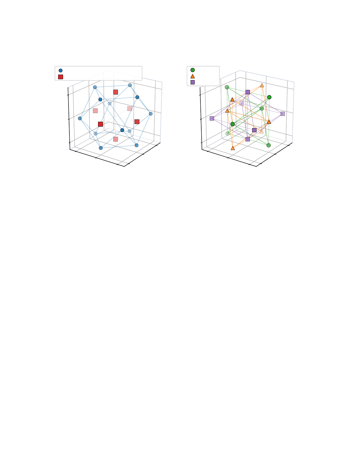
A particle at rest. Figure 2(a) shows the projection: the 12 spatial neighbors form the 𝐷
3
cuboctahedron,
and the 12 time-mixed neighbors project pairwise onto the six axis points. A particle at rest is a worldline
advancing along
𝑥
0
with no net spatial displacement, whose cross-section at any instant is a
𝐷
3
defect of
Ref. [
1
]. Since the lattice has no bond along
(1, 0, 0, 0)
, such a worldline is a zigzag on null bonds, one step
to a neighboring void and one step back, and the explicit operators of Eq.
(6)
are of this form. The five Part I
masses survive the lift unchanged (Section 7).
7
−1
0
1
x
−1
0
1
y
−1
0
1
z
(a) D
4
nearest neighbors projected to 3D:
spatial (D
3
) vs. time-mixed
Spatial NN (D
3
, 12)
Time-mixed NN (12, projected to 6)
−1
0
1
x
−1
0
1
y
−1
0
1
z
(b) Triality decomposition:
three inscribed 16-cells
16-cell A
16-cell B
16-cell C
Figure 2: The 24 nearest neighbors of a
𝐷
4
vertex, projected to 3D by dropping the time coordinate. (a) Spatial
bonds (blue circles, 12 vertices) form the
𝐷
3
cuboctahedron of Ref. [
1
]. Time-mixed nearest neighbors (red
squares, 12 vertices projecting onto 6 axis points) connect adjacent time-slices. (b) The same 24 vertices recolored
by triality. The three inscribed 16-cells (green, orange, purple) interpenetrate at the origin and are permuted
cyclically by triality. The order-three symmetry supplies a distinguished threefold decomposition, proposed as the
transverse generation structure (hypothesis H2, Sections 2 and 6); the mass hierarchy does not follow from this
geometry alone.
3.4. How isotropic is the lattice?
Moments of the bond set. Let
n
1
, . . . , n
24
be the unit vectors along the 24 nearest-neighbor bonds and
define, for even
𝑝
, the moment
𝑀
𝑝
(k) =
Í
𝑗
(k · n
𝑗
)
𝑝
. If
𝑀
𝑝
depends on
k
only through
|k|
the bond set has
no preferred direction at order
𝑝
; a set for which this holds for every
𝑝 ≤ 𝑡
is a spherical
𝑡
-design [
8
]. Odd
moments vanish because the bond set is centrally symmetric. These are statements about a finite vector set,
invariant under the lattice point group and nothing larger; the second moment
𝑆
𝜇𝜈
=
Í
𝑗
𝑛
𝜇
𝑗
𝑛
𝜈
𝑗
is not a tensor
under SO(4) or the Lorentz group, and calling it one, as Part I did, invites a stronger reading than the object
supports. Direct computation gives, for the 12 𝐷
3
bonds and the 24 𝐷
4
bonds respectively,
𝑀
(𝐷
3
)
4
= 3
|k|
2
2
−
𝑖
𝑘
4
𝑖
, 𝑀
(𝐷
4
)
4
= 3
|k|
2
2
exactly, (3)
with
𝑀
2
= 4|k|
2
and
6|k|
2
(script 15 of Ref. [
4
]). The
𝐷
3
shell is a 3-design and no more; the
𝐷
4
shell is a
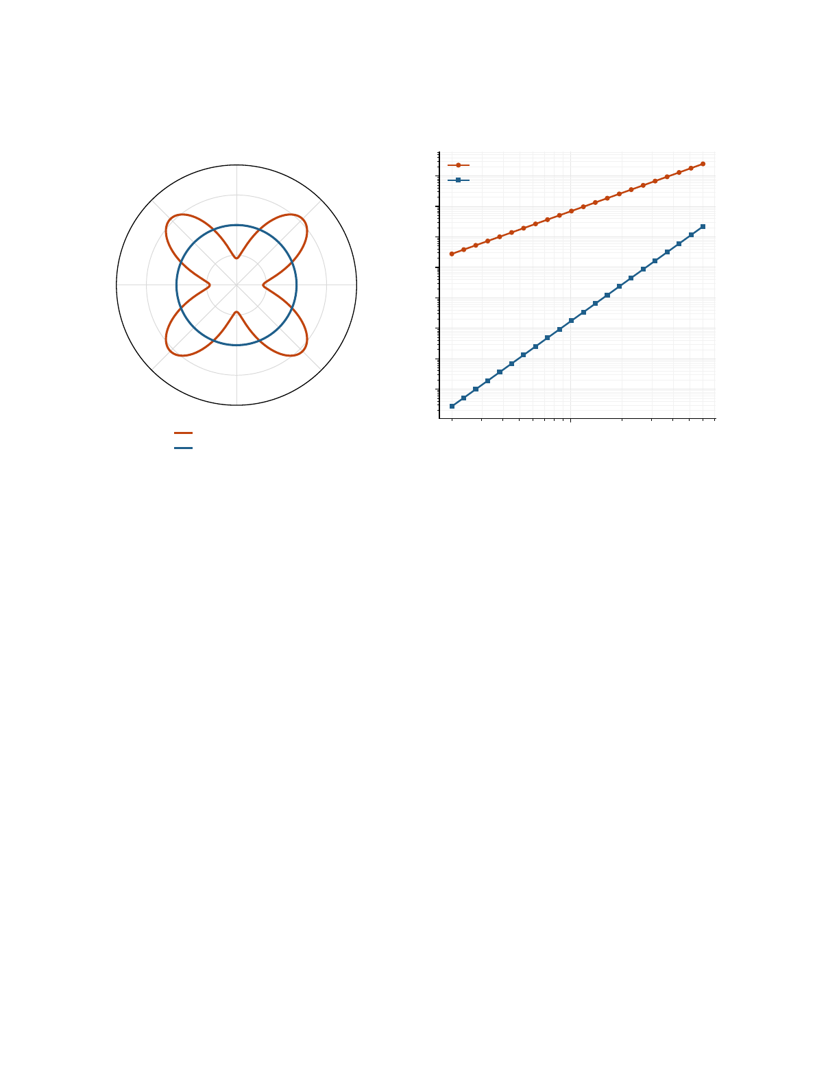
5-design, with its first anisotropy at sixth order (Figure 3(a)). The
𝐷
3
statement supersedes Part I’s reading of
𝑆
𝜇𝜈
∝ 𝛿
𝜇𝜈
as isotropy at all orders; a second moment does not constrain a fourth. Its compatibility conclusion
stands: at optical energies (𝐸/𝑀
𝑃
)
2
≈ 3 × 10
−56
, far below the 10
−20
to 10
−40
bounds of Refs. [9, 10].
Under the foliation. Equation
(3)
is Euclidean: it treats the 24 bonds as equivalent. Under H1 twelve are
spacelike and twelve null, and the physical question is the isotropy of the spatial bond set seen by a mode
on a slice. The
𝐷
3
anisotropy
−
Í
𝑖
𝑘
4
𝑖
is extremal along the coordinate axes, precisely the directions the
cuboctahedron has no bonds along; the null bonds
(±1, ±𝑒
𝑖
)
have spatial parts
±𝑒
𝑖
and point along exactly
8

those axes. With 𝑤 the weight of a null hop relative to a spacelike one,
𝑀
spatial
4
= 3
|k|
2
2
+ (𝑤 − 1)
𝑖
𝑘
4
𝑖
(4)
(script 20 of Ref. [
4
]). In Euclidean signature
𝑤 = 1
by symmetry; in Lorentzian signature it is a property of
the dynamics, the statement that one lattice unit of spatial displacement costs the same on the light cone as
within a slice, which a lattice with a single propagation speed requires. Beside the checkerboard structure of
Section 3.2, this is the second structural reason for the lift: the cuboctahedron cannot be isotropic at fourth
order because it has no bonds along the axes, and the bonds the lift adds along them are the light cone.
The dispersion relation. For a scalar field with nearest-neighbor couplings,
𝜔(k)
2
= 𝜅
Í
𝑗
[1−cos(k ·n
𝑗
𝑎)]
expands in the moments with coefficients
𝑎
2
/2, −𝑎
4
/24, . . .
. The leading term is isotropic on both lattices,
𝜔 = 𝑐
lat
|k|; the first direction-dependent term is the first anisotropic moment, so the fractional spread of the
propagation speed scales as
Δ(𝜔/|k|)
𝜔/|k|
∼
(
(𝑘𝑎)
2
on 𝐷
3
,
(𝑘𝑎)
4
on 𝐷
4
, if 𝑤 = 1; (𝑤 − 1)(𝑘𝑎)
2
otherwise.
(5)
Figure 3(b) confirms the exponents
2.00
and
4.00
from the exact dispersion over a decade in
𝑘𝑎
; at
𝑘𝑎 = 0.1
the spreads are 7 ×10
−5
and 2 × 10
−8
.
What this does not establish. Equation
(5)
is a tree-level kinematic statement about one scalar field on a
fixed lattice. It supplies no renormalization procedure toward a symmetric fixed point; it does not suppress the
loop corrections of Ref. [
9
], which lift Planck-suppressed violation to the percent level unless bare parameters
are tuned to one part in
10
20
, a fine-tuning problem that applies here as it stands; and isotropy is not boost
invariance, which further requires the sign structure
𝐴(𝜕
𝑡
𝜙)
2
− 𝐵|∇𝜙|
2
that assigning a signature does not
produce. For comparison, lattice QCD on
Z
4
, whose 8 bonds are a 3-design with
𝑀
4
= 2
Í
𝑖
𝑘
4
𝑖
, recovers full
Lorentz invariance in the continuum limit despite a maximally anisotropic fourth moment; that recovery rests
on renormalization-group flow, not on design strength, and applies to
𝑘𝑎 ≪ 1
. The defects whose costs are
computed in Sections 7–12.1 are lattice-scale,
𝑘𝑎 ∼ 1
, and no long-wavelength emergence argument covers
them (Section 15.4). The connection to continuum spacetime symmetry is left open (Section 16).
9
k
x
k
y
0.9
1.0
1.1
varies with
direction
exactly
constant
(a) Fourth moment ∑
j
(k ⋅ n
j
)
4
, normalized
D
3
shell (12 bonds)
D
4
shell (24 bonds)
10
−1
dimensionless momentum ka
10
−10
10
−9
10
−8
10
−7
10
−6
10
−5
10
−4
10
−3
spread of ω/|k| over directions
∝ (ka)
2
∝ (ka)
4
(b) Direction-dependence of the propagation speed
D
3
shell
D
4
shell
Figure 3: Direction-dependence of the two bond sets. (a) The fourth moment
𝑀
4
(k)
over directions in a
coordinate plane, each curve normalized by its own mean. The
𝐷
3
shell (12 bonds) varies with direction; the
𝐷
4
shell (24 bonds) is exactly constant, because the 24-cell is a spherical 5-design and the cuboctahedron only
a 3-design. (b) Fractional spread of the phase speed
𝜔/|k|
over directions, from the exact lattice dispersion,
against the dimensionless momentum
𝑘𝑎
. The measured exponents are
2.00
(
𝐷
3
) and
4.00
(
𝐷
4
), matching Eq.
(5)
.
Both panels are computed by
15_spherical_design.py
[
4
] and
gen_fig2_isotropy.py
; neither is drawn
by hand.
4. The Mass-Bearing Code and the Homological Ladder
The verification costs consume f-vector data of the coordination cluster: the sub-complex formed by one
lattice site together with its nearest neighbors and all the cells they span—13 nodes on 𝐷
3
, 25 on 𝐷
4
. What
the cost formulas read off that cluster is its vertex count and its face count. The
𝐷
4
code of Section 3.2, like its
𝐷
3
predecessor, carries vertex stabilizers and void stabilizers—no face stabilizers. This raises a question not
raised in the earlier papers: are the sector counts functionals of any code at all, or are they combinatorial data
external to the error-correcting structure? The answer, established computationally in this section, is that they
are exact stabilizer counts of a second code on the same lattice, and that the two codes play complementary
roles.
4.1. The vertex–plaquette (VP) code
On the vertex–plaquette (VP) code, define qubits on the lattice edges as before, Z-stabilizers on the vertex
stars, and X-stabilizers on all plaquettes—the triangular and square circuits of nearest-neighbor bonds. We
abbreviate it the VP code throughout, to keep it distinct from the
𝐷
4
code of Section 3.2, which carries no
face stabilizers at all. Because every plaquette is a closed loop, it shares an even number of edges with every
vertex star, so the construction is CSS-valid automatically. On
𝐷
3
at
𝐿 = 6
this yields a
[[648, 3]]
code
whose three logical qubits are the torus cycles (verified:
rank(𝐻
𝑍
) = 107
,
rank(𝐻
plaq
) = 538 = 541 − 3
;
10

script 09_code_functional_validation.py [4]).
The detecting-stabilizer count. On this code, define the detecting-stabilizer count of a defect with edge
support
𝑆
as the number of stabilizers associated with the cells of the induced subcomplex of
𝑆
: vertex
stabilizers incident to
𝑆
, and plaquette stabilizers whose support is contained in
𝑆
, filtered by the active sector
of Section 7.1. Evaluated on the Part I defect geometries, this functional reproduces the sector counts exactly:
the pion’s
9 + 8 = 17
(nine incident vertices, eight contained triangles), the muon’s
6
(six contained squares),
the proton’s
13 + 38 = 51
(thirteen vertices, thirty-two triangles, six squares), with the electron’s
𝐶
𝑠
= 1
as
the zero-contained-cells floor. No parameter mediates the comparison. The sector counts of Part I, introduced
there as combinatorial data of the coordination cluster, are thereby shown to be code-native: they are the
literal stabilizer content of the vertex–plaquette code.
How the two codes relate. The two codes on the lattice are directly related. A void stabilizer’s support is an
even subgraph (every vertex of the octahedral frame has even degree), hence a sum of plaquette boundaries:
the
𝐷
4
code’s X-group is a subgroup of the VP code’s. The high-rate code of Section 3 is the VP code with
most face stabilizers omitted, and its logical count measures the omission. The division of labor is then
clean, and we adopt it for the remainder of the paper: the
𝐷
4
code is the topological substrate, carrying the
encoding-rate and distance structure; the VP code is the metric structure, on which verification costs (masses)
are literal stabilizer counts.
4.2. The homological ladder on 𝐷
4
The ladder. The VP construction lifts to
𝐷
4
and extends to a family. The Delaunay decomposition of
𝐷
4
is
the 16-cell honeycomb: at
𝐿 = 4
, exactly
384
cross-polytope 4-cells (
128
centered at odd integer points,
256
at half-odd points), with cell counts
(𝑉, 𝐸, 𝐹
△
, 𝐹
□
, 𝐶
3
, 𝐶
4
) =
𝐿
4
2
, 6𝐿
4
, 16𝐿
4
, 9𝐿
4
, 12𝐿
4
,
3𝐿
4
2
,
every tetrahedron shared by exactly two 4-cells and every triangle by exactly three (verified; scripts
10
–
13
).
Placing qubits on the cells of each dimension in turn, with stabilizers on the adjacent dimensions, yields four
CSS codes whose logical spaces are the cellular homology of the 4-torus:
Qubits on Code 𝑘 Logical content (= Betti number)
edges [[1536, 4]] 4 𝐻
1
: 1 time + 3 spatial winding classes (wt. 4)
faces [[6400, 6]] 6 𝐻
2
: 3 +3 worldsheets under the foliation (wt. 8)
tetrahedra [[3072, 4]] 4 𝐻
3
: membranes (wt. 192 representative)
16-cells [[384, 1]] 1 𝐻
4
: the fundamental class (wt. 384, extensive)
Every parameter was predicted from the honeycomb structure before computation and confirmed by it,
including the diagnosis and elimination of a
2304
-qubit excess traceable to the square-faced 3-cells (script
12). Three consequences restructure the hypotheses of Section 2.
First, the homological placement of the worldlines is settled, and it sharpens H2 rather than discharging it.
The logical space of the edge code is exactly
𝐻
1
(𝑇
4
) = Z
4
2
: one time class and three spatial winding classes.
Two equivalence relations must be kept distinct: inequivalence under the
𝐷
4
code’s stabilizer group (verified
in Section 6.3) and homology in the mass-bearing complex (equivalence modulo plaquette boundaries). The
three triality worldlines separate them: their homology vectors
(𝑤
𝑡
, 𝑤
𝑥
, 𝑤
𝑦
, 𝑤
𝑧
)
are all
(1, 0, 0, 0)
, so they
11

are inequivalent under the
𝐷
4
code yet homologous in the chain complex, all representing the single time
class. That is the physically correct placement, a massive particle at rest wrapping the time circle with no net
spatial displacement, and it holds for every particle worldline: the neutrino is the bare time wrap, the charged
leptons are time wraps carrying transverse structure distinguished by the axis the worldline oscillates along.
Generation structure is therefore finer than homology. The three spatial winding classes are spacelike torus
cycles, not particle worldlines, and their identification is open. For H2 this means the exhaustion component
H2a is not settled by the homology; that the three orbit members have identical verification cost is why
the triality label cannot carry the charged-lepton hierarchy and why flavor must be carried by depth (H2b),
for which a mechanism correlating transverse structure with depth is required and is not contained in the
framework. Both questions are raised in Section 16. The
𝐻
3
classes, which pair with the
𝐻
1
classes one to
one under Poincaré duality, are the conjugate observables of the worldlines rather than defects.
Second, H4a is corrected and then upgraded. For the
𝐷
4
code the dimensional grading is refuted: every
one of its 1282 logical classes reduces to weight
≤ 9
(script 08 of Ref. [
4
]). On the ladder it is exact cellular
homology, with line, surface, volume and bulk classes explicitly constructed. The grading is real and lives
on the chain complex; the identification of the graded classes with the physical sectors (H4b) remains a
hypothesis.
Third, the vertex figure of the honeycomb, computed from the complex, is
(24, 96, 96, 24)
—the f-vector
of the 24-cell. The polytope on which Sections 6–8 are built is not an auxiliary construction; it is the local
structure of the mass-bearing complex at every vertex.
5. Signature and Arrow: The Fifth Axiom
The four earlier axioms still hold. The four axioms of Ref. [
1
] (Minimum Topological Dimension, Sector
Completeness, Boundary Closure, Kinematic Shedding) carry through, with two generalizations. Axiom 1
was originally a spatial statement (
𝑑
spatial
top
≥ 1
), since the
𝐷
3
framework knew no time dimension. With time
now a fourth lattice direction, Axiom 1 reads as a spacetime statement:
𝑑
spacetime
top
≥ 1
. A defect must extend
in at least one direction, but it can extend purely in time. This generalization is the one new ingredient that
admits null worldlines (the neutrino class of Section 9) which would have been rejected by the strict spatial
form. Spatial defects that satisfied the original axiom satisfy the generalized version automatically.
The second generalization concerns Axiom 4. In Ref. [
1
] it was stated for moving point defects, which
shed
𝐷
2
trajectory correlation. The underlying quantity is not specific to trajectories, and we state it in the
form the 𝐷
4
setting requires:
Axiom 4 (Redundancy Shedding). A defect sheds the
𝐷
spatial translations for each independent
vector required to fix its macroscopic embedding in the spatial slice.
Three cases arise in this paper, and the vector count is fixed by the defect’s geometry rather than chosen. A
worldline whose cross-section lies in a single spatial slice is fixed by two vectors, a spatial position and a
kinematic tangent, and sheds
𝐷
2
. A worldline whose tube section engages the null bonds (the depth-3 defect
of Section 8) is fixed by three: position, tangent, and the spatial orientation of its null zigzag, which is a
direction in the slice that a purely spatial cross-section does not possess; it sheds
𝐷
3
. A condensate spans the
whole spatial slice: translating it is the identity, so no position vector enters, and its embedding is fixed by the
𝐷
orthogonal basis vectors that span its extent, shedding
𝐷
𝐷
. The count is a property of the embedding, not
of the particle, and for the three engagement depths of the lepton ladder it reads
𝐷
depth
:
𝐷
1
= 3
at depth 1
(which the electron cannot shed, see below),
𝐷
2
= 9
at depth 2,
𝐷
3
= 27
at depth 3, with the condensate at
the same 𝐷
3
= 𝐷
𝐷
.
12

Why
𝐷
𝑟
and not
𝑟𝐷
. The shedding count is a count of joint correlation labels, not of continuous vector
components. Two embedding vectors carry
2𝐷
real parameters, but the syndrome extraction circuit does
not record parameters; it records, each round, which of the
𝐷
lattice directions each vector’s change points
along. Each independent embedding vector therefore contributes one
𝐷
-valued spatial-direction index, and
for
𝑟
independently correlated vectors the redundant sector of the coupling matrix
𝐵
sector
is labeled by their
Cartesian product,
|{1, . . . , 𝐷}
𝑟
| = 𝐷
𝑟
joint labels, each a syndrome bit that reports embedding rather than
internal structure. This is the sense in which Ref. [
1
] counted
𝐷
2
= 9
“redundant syndrome bits each round”
for a moving point defect, one per (position-direction, tangent-direction) pair; the depth-3 worldline adds a
third index for the direction of its null zigzag and the redundant block becomes
𝐷
3
; the condensate, fixed by
𝐷
basis vectors, gives
𝐷
𝐷
. The exponent counts independent directional indices, and the base is the number
of values each can take.
Two conditions carry over unchanged from Ref. [
1
]. Shedding applies only to free defects: a pinned
worldline’s vertex syndromes report internal structure, not position, and are counted. And a defect can shed
only what it has, so the shedding applies only when
dim(𝐵
sector
)
exceeds the quantity to be shed; the electron,
with
dim(𝐵) = 1
, sheds nothing and keeps
𝐶
𝑒
= 1
. The full enumeration of which candidate defects survive
all five axioms and which fail (the 𝐷
4
analog of Ref. [1]’s 25-candidate sieve) is collected in Section 13.
The remaining three axioms apply to spatial defects exactly as in Ref. [
1
], with “spatial” now meaning the
three directions orthogonal to 𝑥
0
. To fix what 𝑥
0
is, we add one new axiom.
Axiom 5 (Signature and Arrow; hypothesis H1). One coordinate
𝑥
0
of the
𝐷
4
lattice carries Lorentzian
signature. The 12 nearest-neighbor bonds with
Δ𝑥
0
= 0
are spacelike and form the
𝐷
3
sub-lattice of Ref. [
1
];
the 12 time-mixed bonds are null, carry energy and momentum between time-slices, and do not enter the
sector counts of defects whose footprint lies within a slice. The vacuum code state distinguishes the two
orientations of 𝑥
0
: it has an arrow.
Under H1 there is no symmetry to break: the signature distinguishes
𝑥
0
, and the residual symmetry of the
slice, the coordinate permutations
𝑆
3
with the point group of
𝐷
3
, is the one the framework uses. What remains
to fix is the orientation of
𝑥
0
. We model it with a condensate of link variables on the null bonds,
⟨𝑈
null
⟩ ≠ 0
,
⟨𝑈
𝑥
𝑖
⟩ = 0
; there is no bond along
(1, 0, 0, 0)
for a time-axis condensate to sit on. For gauge links the local
expectation value is gauge-dependent, so the condensate must ultimately be characterized gauge-invariantly
(Section 15.4); it is a model of the arrow, not a derivation. Its localized excitation is identified with the
Higgs (Section 12). Below the condensation scale the dispersion reads
𝜔
2
= 𝑚
2
+ 𝑐
2
𝑠
|k
𝑠
|
2
with
𝑚
set by the
condensate; Lorentzian dynamics on the foliation requires in addition the sign structure of Section 3.4, which
is open.
A candidate microscopic bias for the arrow. The axiom asserts an arrow without exhibiting the dynamics
that produces it. A candidate follows from the growth kinematics already in the framework [
3
]: the lattice is
grown, growth happens at a surface, and below that surface the checks are committed while above it they are
pending. The surface distinguishes one direction from the other three by a physical difference in what has
been verified, and a defect worldline couples asymmetrically to its two interlayer directions as a result.
The cost model, and the computation. A defect in a tetrahedral void has interlayer connections to the sheet
below and the sheet above. Hopping destroys bonds to the vertices it leaves and creates bonds to those it
reaches, and every such hop transits an octahedral void, which is an
𝑋
-check site. Creating or destroying a
bond at a vertex whose check is already committed costs a factor
𝑐
in syndrome-free probability, because an
undetermined
𝑍
entering a recorded weight-twelve check flags with probability
1 − 𝑐
; interfaces that are still
pending are free. With
𝑐 =
1
2
and the amplitude per hop
𝐴
2
= 𝑐
𝑛
𝑐
, where
𝑛
𝑐
counts committed interfaces
13

touched, enumeration over all 28 geometric paths gives
𝐴
up
= 0.500, 𝐴
down
= 0.268,
a polarization 𝑃 = (𝐴
up
− 𝐴
down
)/(𝐴
up
+ 𝐴
down
) = +0.302.
The controls are the content. With every check committed, the static crystal, the two cost distributions are
identical and
𝑃 = 0
exactly. With none committed,
𝑃 = 0
with unit amplitudes. With the frontier inverted,
𝑃 = −0.305
. The asymmetry exists if and only if a front exists, and the front fixes its sign. The static case
reproduces this framework’s own centrosymmetry obstruction as a measured zero, which is the check that
matters: a nonzero result there would have indicated an error in the cost model rather than a physical effect.
Varying
𝑐
over
1
4
and
3
4
, costing the octahedral transit, and reversing the void orientation move the magnitude
over
𝑃 ∈ [0.13, 0.54]
and leave the sign and the if-and-only-if character unchanged; nothing below uses the
magnitude.
The growth dynamics thus supplies a candidate bias for the arrow, computable from the stabilizers, and
a falsifier: equal amplitudes under any variation of the cost model would refute it. It does not derive H1:
showing that a front biases the hopping is not showing that the
𝐷
4
vacuum develops the required arrow, let
alone the signature, in its ground state (Section 15.4).
The label is arbitrary; the signature and the shedding count are not. First, the four coordinates of
𝐷
4
are equivalent under the point group, so which of them is written
𝑥
0
is a labeling convention; H1’s content is
that exactly one coordinate carries Lorentzian signature, not which. Second, the kinematic shedding count of
Axiom 4 for a spatial worldline stays at
𝐷
2
= 9
rather than rising to
16
, because the redundancy being shed is
purely spatial trajectory correlation. Time translation generates energy, not a kinematic redundancy. This is
checked directly in Section 7; it constitutes the strongest piece of internal evidence that
𝐷
4
is the correct lift.
6. The 24-Cell, Triality, and the Three-Generation Structure
The local polytope. The 24 nearest neighbors of a
𝐷
4
vertex form the vertex set of a 24-cell centered on
that vertex. Its f-vector is
( 𝑓
0
, 𝑓
1
, 𝑓
2
, 𝑓
3
) = (24, 96, 96, 24),
with Euler characteristic
24 −96 +96 −24 = 0
as required for a closed 4-polytope. Each of the 24 octahedral
3-cells has 6 vertices, 12 edges, and 8 triangular faces. Two octahedral cells meet at each triangular face,
and the 24-cell is the unique regular 4-polytope that is both self-dual and admits the additional symmetry
described below.
6.1. Triality
The threefold split. The 24 vertices partition uniquely into three subsets of 8, each subset forming the
vertex set of an inscribed 16-cell (the regular 4D cross-polytope). Concretely, with coordinates
(𝑥
0
, 𝑥
1
, 𝑥
2
, 𝑥
3
)
as in Section 3.3, the six coordinate pairs {𝑖, 𝑗 } with 𝑖 < 𝑗 split into three pairs of complementary pairs:
𝐴 =
{0, 1}, {2, 3}
, 𝐵 =
{0, 2}, {1, 3}
, 𝐶 =
{0, 3}, {1, 2}
.
Each set contains one pair involving
𝑥
0
and one purely spatial pair. The 8 vertices with nonzero coordinates
in pair set
𝐴
form a 16-cell; the same for
𝐵
and
𝐶
. Triality is the order-3 symmetry that cyclically permutes
these three 16-cells. The corresponding statement in Lie theory is this:
𝐷
4
names the rank-4 simple Lie
14

algebra
𝔰𝔬(8)
, whose simply connected group is
Spin(8)
, and triality is the order-three outer automorphism
of that group [
12
]. It has no analog in any other dimension. We use “
𝐷
4
” for the lattice throughout and name
the algebra and group explicitly whenever they are meant, since the same symbol serves both. The geometric
realization in the 24-cell of 𝐷
4
is its only finite-dimensional manifestation.
Figure 2(b) shows the three 16-cells in the 3D projection, with their edges drawn in different colors. Each
16-cell is at distance 0 from the origin (they share the common center) and is mapped to the next by an outer
triality rotation.
6.2. Why exactly three generations
A worldline defect can participate in the triality decomposition at three levels: localized within one 16-cell,
engaging the spatial halves of all three, or engaging all three in both halves. The third engages the full 24-cell,
so no further level exists within this ladder. The three levels are constructed; that they exhaust the admissible
charged-lepton structures is hypothesis H2a, and Section 4.2 shows that all three lie within the single time
class of the mass-bearing complex, so exhaustion is a statement finer than homology and remains open. The
order-three automorphism, verified below, acts separately: it cycles the three 16-cells, and with them the
anchoring of any depth-1 worldline; for a charged edge the three anchorings are identified as one electron
(H2c), for a null worldline they are the three neutrino flavors (Section 9). It does not by itself count generations.
Conditional on H2a the framework predicts three generations of leptons and, by the same reasoning at the
hadronic level, of quarks. The LEP measurement of the invisible Z width,
𝑁
𝜈
= 2.996 ± 0.007
[
13
], is
consistent with three and incompatible with two or four; a fourth light neutrino would falsify H2a.
6.3. Triality as a code automorphism
Triality is a symmetry of the polytope; the framework’s content sits in the code, so triality must act as a
symmetry of the code. Let
𝜋 : (𝑥
0
, 𝑥
1
, 𝑥
2
, 𝑥
3
) → (𝑥
0
, 𝑥
2
, 𝑥
3
, 𝑥
1
)
be the coordinate 3-cycle fixing the time axis.
The verification script
05_triality_code_automorphism.py
of Ref. [
4
] confirms the following at
𝐿 = 4
:
1. 𝜋
has order three, fixes the time coordinate distinguished by Axiom 5, and cycles the three 16-cell
triality sets as
𝐴 → 𝐶 → 𝐵 → 𝐴
with exactly 8 nearest-neighbor edges in each transition (matching
the 8 + 8 + 8 = 24 decomposition).
2. 𝜋
is a code automorphism of the
𝐷
4
CSS code: the lattice permutations on
𝐷
4
vertices (vert_perm) and X-
stabilizer sites (xsite_perm) and the induced permutation on edges (edge_perm) satisfy
𝐻
𝑍
[vert_perm][:
, edge_perm] = 𝐻
𝑍
and
𝐻
𝑋
[xsite_perm][:, edge_perm] = 𝐻
𝑋
. That is, applying triality permutes the
Z- and X-stabilizer groups among themselves rather than mapping any stabilizer outside the group.
3.
The orbit structure of
𝜋
on the qubit set has no fixed points: every one of the 1536 qubits sits in a size-3
orbit, for a total of 512 orbits. Triality is non-trivial on every physical qubit.
The triality label then becomes concrete at the level of logical operators. We construct three explicit closed
worldlines
wl
𝐴
, wl
𝐵
, wl
𝐶
, each anchored in one of the three triality sets and wrapping the time direction on
the 𝐿 = 4 torus via four nearest-neighbor steps:
wl
𝐴
: (1, 1, 0, 0) → (1, −1, 0, 0) → (1, 1, 0, 0) → (1, −1, 0, 0),
wl
𝐵
: the same with steps in the (0, 2) plane, wl
𝐶
: in the (0, 3) plane.
(6)
Each is a Z-string of weight 4, supported on edges of a single triality set. The verification script confirms:
15

•
All three worldlines commute with every X-stabilizer (
𝐻
𝑋
· wl
𝑖
= 0 (mod 2)
), so they are valid logical
Z candidates.
• None lies in the row-span of 𝐻
𝑍
, so all three are genuine logical operators rather than stabilizers.
• The triality permutation cycles them: 𝜋(wl
𝐴
) = wl
𝐶
, 𝜋
2
(wl
𝐴
) = wl
𝐵
, 𝜋
3
(wl
𝐴
) = wl
𝐴
.
•
The pairwise differences
wl
𝐴
+ wl
𝐵
,
wl
𝐴
+ wl
𝐶
,
wl
𝐵
+ wl
𝐶
are not in the row-span of
𝐻
𝑍
. The three
worldlines therefore represent three inequivalent logical operator classes of the CSS code, related by a
code automorphism.
Three inequivalent logical operators forming one orbit under the order-three automorphism is the code-level
realization of the triality label. These particular operators have no spatial cross-section: they are the bare time
wraps of Section 4.2, the null worldlines of Section 9, and the orbit is the neutrino triplet. For a charged
lepton the same label is the 16-cell containing its spatial cross-section (H2c); the generations are the three
engagement depths, not the three orbit members. The order of the automorphism fixes the size of the orbit,
not the number of admissible worldline structures (H2a), and the three operators are homologous in the
mass-bearing complex (Section 4.2), so what distinguishes them is finer than homology. The same operators
arise for any anchor in the orbit by translation invariance; a complete classification by triality orbit and cellular
class is open.
Three labels, and how they map. The triality label indexes which 16-cell component(s) a worldline’s
support selects; the engagement depth is its level of participation (Section 6.2); the flavor names the particle.
Depth is what the mass formulas consume (Table 2). The triality decomposition supplies three components
and the support hierarchy three levels; that the two counts coincide is a property of the constructed ladder, not
of the automorphism’s order, and is part of H2a. At depth 1 the label selects one of three symmetric choices
(H2c, the quotient identifying them); at depths 2 and 3 the support is symmetric across the three and the label
is not used.
7. Worldlines and the Spatial Predictions
From static defects to worldlines. In Part I a particle at time
𝑡
was a defect geometry in 3-space, and its rest
mass was the verification cost of that geometry. In
𝐷
4
a particle is a worldline through 4-space. A particle at
rest corresponds to a worldline with no net spatial displacement, a null zigzag advancing along the time axis
(Section 3.3); a particle with 3-velocity
v
corresponds to a worldline tilted by
tan
−1
(|v|/𝑐)
relative to that axis.
Cost of a worldline. The verification cost of a worldline is defined over a tubular spacetime neighborhood
of one proper-time step: the edges entering
𝐸
𝑠
are those of the defect’s coordination structure within the tube.
The tube formulation is needed for uniformity, because depth-3 defects engage time-mixed bonds that lie in
no fixed-time slice (Section 8). For a worldline aligned with the time axis whose coordination structure is
purely spatial, the tube count reduces to the fixed-time spatial cross-section (exactly an
𝐷
3
defect) and the
cost reduces to the Part I formula
𝐶
worldline at rest
𝑥
= 𝐶
𝐷
3
spatial cross-section
𝑥
.
The Landauer–Einstein relation [
17
] and the cancellation of
𝑘𝑇 ln 2
in mass ratios both carry through
unchanged. So all five Part I predictions are preserved:
𝐶
𝑒
= 1, 𝐶
𝜇
= 207, 𝐶
𝜋
±
= 273, 𝐶
𝑝
= 1836, 𝐶
𝑛
= 1839,
matching the experimental ratios 𝑚
𝑥
/𝑚
𝑒
to within 0.008–0.12 % as before.
16

The consistency check. It concerns Axiom 4. The muon’s formula reads
𝐶
𝜇
= 𝐸
𝑠
×𝐶
𝑠
−𝐷
2
= 36×6−9 = 207
.
If
𝐷
2
had to be re-interpreted as
4
2
= 16
in the 4D theory, the muon would come out at
216 − 16 = 200
,
missing the empirical value of 206.77 by
3.3%
—far outside the framework’s accuracy. Axiom 5 is what
keeps
𝐷 = 3
: kinematic shedding subtracts spatial trajectory correlation, not time translations. The match at
𝐷
2
= 9 is therefore strong internal evidence that the 𝐷
3
sub-lattice is the correct “spatial slice” of 𝐷
4
.
7.1. The sector map from worldline kinematics
Part I assigns each particle an active stabilizer sector (which of
𝑉
,
𝐹
△
,
𝐹
□
enter
𝐶
𝑠
) but do not derive
the assignment. In three dimensions no derivation is possible: the muon and the proton occupy the same
36-edge coordination footprint, with identical boundary structure (12 odd-incidence vertices; verified by
07_sector_map.py
[
4
]), yet carry different sectors. Any rule that reads the sector off the spatial footprint
must assign them the same one.
Pinned and free worldlines. The
𝐷
4
lift supplies the missing information. A defect’s worldline is either
pinned to the time axis (confined states, whose color-flux structure anchors them) or free (deconfined states,
whose worldline tilt encodes motion, as above). For a free worldline, the vertex syndromes recorded at
successive extraction rounds report only the defect’s changing position—they are trajectory correlates in
precisely the sense of Axiom 4, which mandates that such syndromes be shed from the verification cost. For a
pinned worldline they report internal color structure and must be counted. This yields the
Worldline sector rule. The vertex sector
𝑉
belongs to the active sector
𝜎
if and only if the
worldline is pinned; for free worldlines the vertex syndromes are kinematic and are shed.
The rule reproduces all seven sector assignments in play, the five of Part I (electron, muon, pion, proton,
neutron) and the two of this paper (tauon, neutrinos) (verified by
07_sector_map.py
[
4
]). The diagnostic
pattern is sharper than mere agreement: the two particles that every footprint-based rule misclassifies, the
electron and the muon, are exactly the free-worldline states—the cases in which the trajectory-shedding
mechanism operates. The 3D projection fails precisely where the 4D kinematics carries the information.
Together with the
𝐷
2
= 9
dimension check above, this constitutes strong internal evidence that
𝐷
4
is the
correct lift: the sector map is underivable in the 3D framework and reproduced by the worldline rule in the
4D one.
What the sector rule does not yet prove. The rule is established here as a consistency result across the
seven assignments; a first-principles calculation showing that the vertex bits of a tilted worldline carry position
information only (for instance, that the mutual information between successive-round vertex syndromes and
the worldline tilt saturates the syndrome entropy for a minimal moving defect) remains open and is listed in
Section 16. And the residual
𝐶
𝑠
= 1
of the electron, the single bit that survives shedding, is interpreted as the
defect’s existence bit; the rule motivates this interpretation but does not force it.
8. The Tauon and the Three Charged Leptons
Order of the derivation. Nothing in this section or in Section 12 refers to experiment, and the order is
deliberate. First the structure is established: the triality decomposition of the 24-cell into three 16-cells
and the engagement hierarchy built on it (Section 6.2) give a nested ladder of exactly three depths for a
17

charged worldline, and that the constructed ladder has three rungs and terminates at the third is a statement
about the lattice, verified by enumeration before any count is taken. That these three exhaust the admissible
charged-worldline structures is not derived; it is hypothesis H2a, stated in Section 2, and the claim that there
are exactly three charged leptons is conditional on it. Only then is each depth’s verification cost assembled, by
the rules of Section 7.1 and Axiom 4 as they stand, with the conventions of Part I applied unchanged. The
comparison with experiment is made only after every count in the paper has been fixed, in Sections 14 and 15.
The same order governs the Higgs: Axiom 5 requires a condensate for the arrow; its localized excitation is a
defect whose footprint the lattice fixes (
𝐾
3
and
𝐷
, Section 12.1); conditional on the resolution lemma of H5,
its cost follows from that footprint and the same shedding grammar. A reader who covers Section 15 and the
deviation columns of Section 14 should be able to reproduce every integer in the paper from the lattice alone.
Table 2 fixes what the three depths mean.
Table 2: The three engagement depths. “Cross-section” is the slice through the worldline at an instant of proper
time; “16-cells engaged” counts how many of the three triality components the tube section touches, and whether
it touches their spatial halves only or both halves. The cost column applies the worldline sector rule of Section 7.1
together with Axiom 4. That rule fixes the vertex sector; the full set of four sector rules, which the sieve needs, is
stated in Section 13.
Depth Tube section 16-cells engaged Active sector 𝐶
𝑥
1 single 𝐷
3
edge one, fractionally trivial (𝐶
𝑠
= 1) 1
2 𝐷
3
3-sheet all three, spatial halves 𝐹
□
= 6 36 × 6 − 9 = 207
3 full 24-cell mod 𝑇 all three, both halves 𝐹
□
= 45 (H3) 78 × 45 − 27 = 3483
8.1. Electron: depth 1
The electron is a worldline whose spatial cross-section is a single
𝐷
3
edge—the minimum 1-sheet defect of
Ref. [
1
]. By triality, the cross-section is localized within a single 16-cell sub-structure of the local 24-cell.
With 𝐸
𝑠
= 1 and trivial sector 𝐶
𝑠
= 1,
𝐶
𝑒
= 1 × 1 = 1.
8.2. Muon: depth 2
The muon worldline engages the spatial halves of all three 16-cell sub-structures. Its spatial cross-section is
the full
𝐷
3
3-sheet (the 13-node cluster), with only the EM sector active and the state deconfined so Axiom 4
applies:
𝐶
𝜇
= 𝐸
𝑠
×𝐶
𝑠
− 𝐷
2
= 36 × 6 − 9 = 207.
This is identical to the Part I derivation; the new interpretation is that the
𝐷
3
3-sheet defect engages the
spatial halves of all three triality sub-structures simultaneously. The 12
𝐷
3
nearest-neighbor bonds split as 4
bonds in each of the three triality sets—the spatial pair from each pair-of-pairs
{(0, 1), (2, 3)}
,
{(0, 2), (1, 3)}
,
{(0, 3), (1, 2)}
contributes its purely-spatial coordinate pair
(2, 3)
,
(1, 3)
,
(1, 2)
respectively. The 3-sheet
therefore touches all three 16-cells, but only on their spatial halves, leaving the time-mixed halves uninvolved.
We call this configuration “depth 2” to mark its intermediate position between depth 1 (a single edge touching
one 16-cell fractionally) and depth 3 (the full 24-cell touching every 16-cell in both halves).
18

8.3. Tauon: depth 3
The tauon worldline engages all three 16-cell sub-structures simultaneously. Its proper-time tube section is the
full 24-cell of
𝐷
4
—all 24 nearest neighbors of the central node, including the 12 time-mixed bonds, which
lie in the spacetime tube though in no fixed-time slice (Section 7). This is why the tube formulation of the
worldline cost is required: the electron and muon tube sections happen to be purely spatial; the tauon’s is not.
We need to identify the EM sector in the 24-cell.
The square count does not lift as a face count. The 24-cell has 96 triangular 2-faces, but no square 2-faces.
The cuboctahedron’s
𝐹
□
count of 6, which gave the muon’s factor of 6, does not lift as a face count—one
needs a different identification of the EM sector. The natural generalization is the count of planar 4-vertex
configurations whose four sides are polytope edges (on the cuboctahedron they coincide with its square
2-faces, which is why both counts gave 6 in Ref. [
1
]). Direct enumeration on the 24-cell yields 72 such
squares: each pair of vertices at distance 2 has exactly four common nearest neighbors among the 24-cell
skeleton, two of which themselves form a distance-2 pair, giving 2 squares per diagonal pair and
72 ×2/2 = 72
distinct squares in total. The script 02_24cell_triality.py [4] enumerates these explicitly.
The 24-cell under the foliation is a causal diamond. By Section 3.3 the tube section is not a ball of 24
equivalent neighbors. It is the spatial cuboctahedron (12 vertices, 24 shell edges, the 6 squares of the muon),
a future light-cone shell of 6 vertices forming an octahedron (12 edges among them, 3 squares), a past shell
of the same shape, and 48 null edges joining the cone shells to the cuboctahedron; the 72 squares sort as 6
spatial, 24 with two future vertices, 24 with two past, 3 in each cone shell, and 12 straddling past to future
through two spatial vertices. Figure 1 gives the Euclidean incidence structure these counts are drawn from.
The time-reversal identification. H3 states that a causal extraction circuit verifies one member of each pair
of objects exchanged by
𝑇 : 𝑥
0
↦→ −𝑥
0
. On the diamond,
𝑇
fixes the cuboctahedron pointwise and swaps
the two cone shells. Counting orbits (
20_lorentzian_signature.py
[
4
]): the 96 shell edges fall into 60
orbits (24 spatial edges fixed; 24 future–spatial paired with 24 past–spatial; 12 future–future paired with
12 past–past), the 24 spokes into 18 (12 spatial fixed, 6 pairs), and the 72 squares into 45 (6 spatial and 12
straddling squares fixed;
24 +24 → 24
;
3 +3 → 3
). The same map acting on the muon’s cuboctahedron fixes
every edge, spoke and square: the identification changes nothing there, which is why Part I never encountered
it.
The depth-3 count then follows by the muon’s rule, with the muon’s conventions and the depth-3 shedding
of Axiom 4:
𝐶
𝜏
= 𝐸
𝑠
× 𝐹
□
− 𝐷
3
= (60 + 18) × 45 − 27 = 78 × 45 − 27 = 3483. (7)
This closes the derivation of the charged-lepton ladder. The three counts
1
,
207
and
3483
follow from the
depth variable, one counting convention applied identically at every depth, the identification H3, and the
shedding exponent of Axiom 4, with no reference to any measured mass. The comparison with experiment is
deferred to Section 15.
Why time reversal and not inversion. The 24-cell is centrally symmetric, and inversion
v ↦→ −v
also pairs
its objects antipodally, so one might ask why the identification is not taken under inversion. Inversion is the
wrong map for a foliated lattice. It reverses space as well as time, so it is not a symmetry that respects the
foliation of H1: it does not fix the spatial slice, and applied to the muon’s cuboctahedron it would halve the
muon’s squares and spokes as well, which Part I never did. Time reversal is the map the foliation singles
19

out: it fixes every spatial object, so it is invisible to every Part I defect, and it pairs exactly the objects a
causal circuit cannot verify independently. Under it one rule serves both leptons; the inversion alternative is
tabulated in Section 14.
9. Neutrinos as Null Worldlines
Why neutrinos were missing. Part I had no place for neutrinos. The electron was the minimum stable defect
at
𝐶
𝑒
= 1
, and any neutrino with
𝑚
𝜈
/𝑚
𝑒
< 2 × 10
−6
would require
𝐶
𝜈
< 10
−6
, far below the topological
floor of one bit. The Part I defect classification contained no configuration in this regime.
Null worldlines.
𝐷
4
under H1 offers a new class of defect: a worldline whose spatial cross-section is empty.
Such a defect has no
𝐷
3
presence at any instant, but it represents a real topological obstruction in the time
direction. It engages only the 12 null bonds, not the 12 spatial ones. Since the lattice has no bond along
(1, 0, 0, 0)
, the worldline is a path on the light cone: each step moves one slice forward and one unit along a
coordinate axis, from a
𝐷
3
site to a void or back. A path that never reverses its spatial direction moves at the
lattice speed of light; a path that reverses has a rest frame, and the rate of reversal is what distinguishes it from
a massless mode. This is the structure of the Feynman checkerboard, and it gives the accumulated cost over a
worldline segment of proper time 𝜏 the form
𝐶
𝜈
(𝜏) = 𝛼
𝑡
𝜏,
with
𝛼
𝑡
the verification cost per reversal times the reversal rate. The instantaneous spatial verification cost is
zero because there is no spatial cross-section to verify; the reversals are the only events the code can register.
Because the null links are condensed (Axiom 5),
𝛼
𝑡
is suppressed relative to the unbroken-phase rate by the
condensate density, so the neutrino mass is parametrically small,
𝑚
𝜈
𝑚
𝑒
∼ 𝛼
𝑡
≪ 1,
with the value of
𝛼
𝑡
depending on the condensate scale (the Higgs vacuum expectation value, VEV) and not
determined by topology alone. The framework thus predicts that neutrinos are much lighter than the electron
without fixing the absolute scale.
Status. The null worldline operator is explicitly constructed: the three time-wrapping operators of Section 6.3,
the bare time wraps of Section 4.2, are weight-4 zigzags of four null bonds with two reversals. Because they
are logical they commute with every stabilizer and fire no local syndrome—the structural fact that sets the
spatial verification cost to zero also renders them nearly invisible to the code, a suggestive match to neutrino
phenomenology. But it also means that detectability rests entirely on the time-direction channel, and
𝛼
𝑡
is
not computed. The neutrino sector is therefore a qualitative proposal within the framework: its three-flavor
count follows from the triality anchoring (conditional on H2), and its mass mechanism is a program, not a
prediction.
By triality, null worldlines come in three flavors, one per 16-cell:
𝜈
𝑒
↔ 16-cell 𝐴, 𝜈
𝜇
↔ 16-cell 𝐵, 𝜈
𝜏
↔ 16-cell 𝐶.
The Pontecorvo–Maki–Nakagawa–Sakata (PMNS) mixing matrix is proposed to arise from triality rotations
between these three 16-cells; a derivation of the mixing angles requires a mechanism coupling the triality
sectors, which the framework does not contain (Section 16).
20

Three qualitative expectations follow under H2 and the hypothesized time-direction channel. (i) There are
exactly three light neutrino species (Section 6.2). (ii) All three are far lighter than the electron,
𝑚
𝜈
≪ 𝑚
𝑒
,
consistent with current bounds
𝑚
𝜈
< 1 eV
. (iii) Generation mixing is nontrivial, with mixing angles related
to triality rotations. The framework cannot yet predict the absolute mass scale, but the qualitative picture is
fixed, and the checkerboard reading makes the missing quantity concrete:
𝛼
𝑡
is a reversal rate on the null
lattice, listed in Section 16.
10. Gauge Bosons as 2D Worldsheets
Part I recovered the Standard Model (SM) gauge boson count structurally: the 12
𝐷
3
nearest-neighbor bonds
partition as
𝐾
3
= 8 + 4
, matching 8 gluons plus the four electroweak bosons; the time-mixed bonds contribute
Wilson-line phases [
16
] rather than further bosons, and the Higgs is a scalar order parameter treated in
Section 12. The masses themselves were excluded as “involving the Higgs mechanism.” The
𝐷
4
construction
permits treating the gauge bosons as genuine topological defects.
Why gauge bosons are 2D objects. A gauge field
𝐴
𝜇
is a 1-form. Its field strength
𝐹
𝜇𝜈
is a 2-form. The
natural lattice realization of a 2-form is a two-dimensional defect—a worldsheet, not a worldline. Worldsheets
exist as proper extended objects only in spacetime dimension
≥ 4
: in 3D a 2D defect has codimension 1 and
partitions space into halves, which is too restrictive.
𝐷
4
is the minimum-dimensional setting in which gauge
bosons can be realized as topological defects in the same sense that fermions are realized as worldlines.
The scope of this section should be fixed before the constructions: what follows is a proposed geometric
correspondence, conditional on the sector identification H4b, not a derivation of the gauge sector. Representa-
tions, structure constants, interactions, helicities, and gauge redundancies are not obtained here; the
8 + 4
bond partition matches the gauge boson count structurally but does not derive the group SU(3)
×
SU(2)
×
U(1).
For the photon the correspondence is supported by the enumerated kinematic argument of Section 10.1,
which establishes what a massless vector mode requires but is not a proof that the physical photon is exactly
massless.
10.1. Photon: 𝐶
𝛾
= 0
The photon costs nothing to verify, and the reason is a property of the lattice. Under H1 it has a name before
any counting: the
⟨100⟩
links from a
𝐷
3
site to its six neighboring voids are the spatial shadow of the null
bonds (Section 3.3), so a field carried by those links is carried by the light cone. What follows establishes by
enumeration that this sector has the kinematic structure a Maxwell field requires.
Method. With
𝐶
𝑝
the
𝑝
-cochains on a sublattice and
𝑑
𝑝
the coboundary, a one-form gauge field is an
element of
𝐶
1
and the Hodge decomposition
𝐶
1
= im 𝑑
0
⊕ im 𝑑
⊤
1
⊕ H
1
splits it into pure gauge, physical
and harmonic parts; the physical polarization count is
dim(im 𝑑
⊤
1
)
per site, computed by exact elimination
(script 17 of Ref. [
4
]). Two lattice properties then sort the sublattices of the packing without ambiguity
(Table 3, Figure 4): bipartiteness, which the height construction of an emergent U(1) photon requires, and
centrosymmetry of the bond star, which decides whether strain couples to the gauge potential at leading order.
Result. The
⟨110⟩
network is non-bipartite and its one-form sector carries one propagating polarization
per site: its two-cells are the octahedral voids, of which there are as many as sites, so
im 𝑑
0
and
im 𝑑
⊤
1
have
equal dimension. The
⟨100⟩
links form a simple cubic lattice that is bipartite, and a one-form field on them
has one pure-gauge and two transverse modes per site: at
𝐿 = 4
the per-site ranks are
0.984
exact and
1.969
coexact, at
𝐿 = 6
they are
0.995
and
1.991
, and the harmonic dimension is
3 = 𝑏
1
(𝑇
3
)
at both sizes. That
21
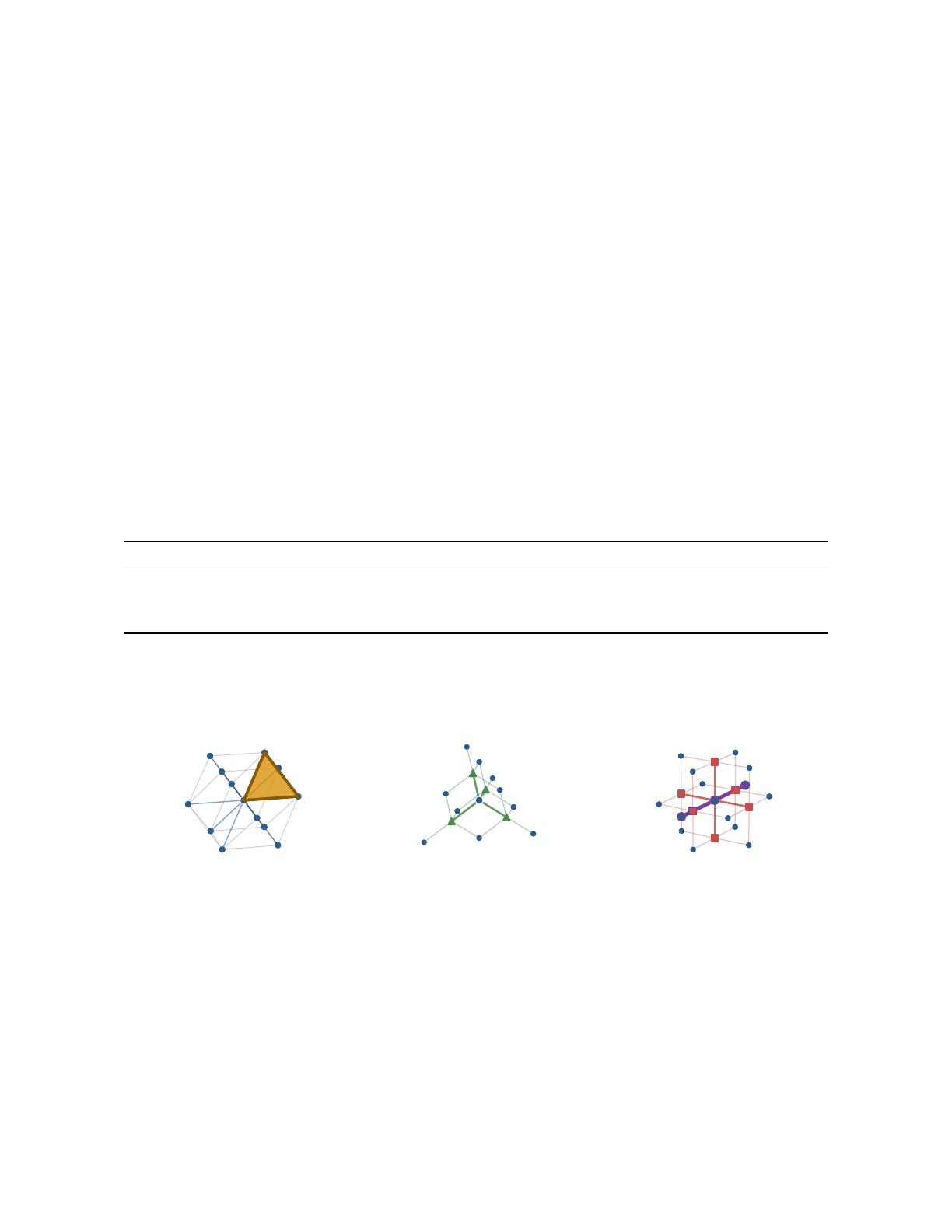
star is centrosymmetric, so its rank-three moment vanishes and no piezoelectric channel sources the gauge
potential at leading order. Together these give the
⟨100⟩
sector the structure required for a Maxwell-like
massless mode, two transverse degrees of freedom with no leading strain coupling, which is stronger than
the bundle-triviality argument it replaces because each part is enumerated, and weaker than a proof of
masslessness: centrosymmetry forbids the rank-three coupling but not every mass-generating mechanism.
The identification
𝐶
𝛾
= 0
,
𝑚
𝛾
= 0
remains conditional on the gauge-sector correspondence; the experimental
bound is 𝑚
𝛾
< 10
−18
eV.
The gauge field does not disturb the code, and matter couples without an added interaction. A
⟨110⟩
code
edge joins two even sites; a
⟨100⟩
link joins an even site to an odd one; at
𝐿 = 4
there are 192 of each and
they share none, so the two operator algebras commute trivially. Coupling arises because the step
(1, 1, 0)
is the composition of
(1, 0, 0)
and
(0, 1, 0)
through an odd site, an octahedral void: all 648 edges at
𝐿 = 6
,
traversed in both directions, are each covered by exactly two two-step
⟨100⟩
paths with a void intermediate
(script 18 of Ref. [
4
]). A defect moving along a code edge accumulates the product of two link phases; the
two covering paths of an edge close a unit cubic plaquette, and the phase is defined only up to the flux through
it: the ambiguity is the field strength the defect radiates into, which is what a gauge coupling is.
Table 3: The three sublattices of the packing sorted by the two criteria. Bipartiteness decides whether the height
construction of an emergent U(1) photon is available; centrosymmetry of the bond star decides whether strain
couples to the gauge potential at leading order. Only the
⟨100⟩
links satisfy both, and only they carry the Maxwell
count.
Sublattice Coordination Bipartite? Centrosymmetric? Polarizations Sector
⟨110⟩ nearest neighbor 12 no yes 1 code, color
⟨111⟩ diamond 4 yes no — —
⟨100⟩ node–void 6 yes yes 2 electromagnetism
(a) ⟨110⟩ nearest neighbors
K = 12, non-bipartite: no photon
(b) ⟨111⟩ diamond
K = 4, bipartite, not centrosymmetric
(c) ⟨100⟩ simple cubic
K = 6, bipartite: Maxwell
odd cycle propagation path
Figure 4: The three sublattices, drawn from computed geometry. (a) The
⟨110⟩
nearest-neighbor shell, a
cuboctahedron; its triangular faces are odd cycles, so the bipartite height construction underlying the emergent
𝑈(1)
Coulomb mode is unavailable on this network. This does not by itself imply color confinement; Section 10
locates confinement’s entry into the cost in the sector rule and the separation potential in the geometry of Ref. [
3
].
(b) The
⟨111⟩
diamond sublattice, bipartite but not centrosymmetric. (c) The
⟨100⟩
links to the octahedral voids.
Nodes (circles) and voids (squares) together form a simple cubic lattice, bipartite by parity, with the highlighted
path showing how the field propagates: it alternates between the two site types and never breaks, because every
even site has an odd neighbor one step along each axis. The three share sites; (a) and (c) share no bonds.
The vanishing photon cost is thus a consequence of an enumerated polarization count and a vanishing
22

point-group moment, both checkable without reference to this framework.
10.2. Gluons: paired color, the sector rule, and the located link phases
The color sector is carried by the triangular plaquettes of the
⟨110⟩
network (rule R2), the eight triangular-
plaquette bonds of Part I’s
12 = 8 + 4
partition and the eight triangular faces on which Ref. [
3
] places the
gluon channels; the chordless hexagons of the
{111}
planes, each bounding six of those triangles, are the
six-cycles on which the link construction below is carried out. What the code says about color before any
gauge dynamics is placed on it can be computed, and we do so here on the
𝐷
3
code of Ref. [
2
], which is the
spatial slice of the present lattice; every number is reproduced by script 21 of Ref. [4].
Method. (i) A parity count. Every edge has two endpoints (
𝐻
𝑍
column weight 2) and lies in exactly two
octahedra (
𝐻
𝑋
column weight 2), so any Pauli operator anticommutes with an even number of vertex checks
and an even number of void checks. The statement is tested exhaustively on the
4
6
− 1 = 4095
non-identity
Pauli operators supported on a chordless
{111}
hexagon, which bounds six of the triangular color channels.
(ii) A link construction. The dipole template of the photon is transplanted to a hexagon: the
𝑋
-supports on its
six edges charged at an antipodal vertex pair are enumerated, their difference is tested against the
𝑋
-stabilizer
group, and the three antipodal pairs are composed.
Result. (i) All 4095 operators have even vertex and even void syndrome, and none flips exactly one
vertex check. Since every component of an
𝔰𝔲(3)
-valued link candidate is a Pauli string, no single-endpoint
color-charged link exists on the strong channels or anywhere else: color charge comes in pairs, by the
same parity argument that makes the electromagnetic sector dipolar. This is Gauss’s law on the code, not
confinement; it says charge is paired, not that a pair cannot be separated. (ii) Exactly two 𝑋-supports on the
hexagon are charged at a given antipodal pair, the two half-hexagon arcs of weight 3, each disturbing six void
checks; their difference is the hexagon loop, which lies outside the
𝑋
-stabilizer group, so the phase between
the two routes is physical and the gluon-field degrees of freedom sit on the hexagon loops, as the photon’s
sit on the void four-cycles. The three antipodal pairs of one hexagon are the three color directions; their
strings pairwise overlap on edges in every orientation, so their phases cannot be independently diagonalized,
and composing one route per pair gives, in all eight orientation assignments, not the neutral loop but the
alternating edge triple, three disjoint edges charging all six vertices.
What the sector rule prices. Confinement enters the cost through the sector rule. The proton and the muon
share the same footprint, the 36 edges of the 3-sheet cluster, and differ in cost because a free colorless defect
activates the six square faces,
36 × 6 = 216
before shedding, while a confined one activates its full sector
of
13 + 38 = 51
checks,
36 × 51 = 1836
, since a confined state cannot ignore any check able to detect it
(Axiom 2 and rule R4). The difference is a statement about which checks a confined state must satisfy; it is
not a binding energy, and no correspondence with the QCD decomposition of the proton mass is claimed or
available. In QCD the proton is three light quarks and a field energy that supplies nearly all of the mass; in
this framework the proton is a single trapped node, its three valence bonds are the quarks of Ref. [
3
] (carrying
the charge thirds by projection) and its three colors are the skew-edge pairs of the bounding tetrahedron, so the
quarks are bonds of a single defect rather than defects of their own, the framework assigns them no separate
mass (the individual quark masses are among the quantities it does not predict, Section 15), and the baryon
mass is one count. The framework has no analog of a constituent-plus-binding decomposition, and the sector
rule that produces the count is a consistency result across the assignments of Section 7.1, not a first-principles
derivation.
What the code does not fix. It does not fix the cost of separating color sources. Definition 1 of Part I,
𝐶 = dim 𝐵 = 𝐸
𝑠
×𝐶
𝑠
, is justified by the hook-error argument on a compact footprint, where every qubit lies
within extraction reach of every detecting stabilizer and every pair must be verified; that premise is what
23

makes the product the count, and it is the premise under which every mass in this paper is computed. A color
string between separated sources is not a compact footprint, so the argument that produced the definition
does not cover it, and the framework fixes no verification cost for an extended object; no claim of this paper
rests on one. The potential between separated sources is derived in the geometric layer of Ref. [
3
]: a trapped
node’s valence bonds cannot be extracted from its void without stretching past the exclusion length
𝐿/
√
3
against the restoring pull of the surrounding
𝐾
3
= 12
shell, and the cost grows linearly with displacement,
𝑉 = 𝜎𝑟
, with
𝜎
set by the bond energy. The confined state is priced by the code; the string that would pull it
apart is priced by the geometry.
What this does not establish. A dynamics: the phases on the hexagon loops are located but nothing
acts on them. Nor a binding energy: the sector rule prices a confined state, not the binding of constituents.
Non-bipartiteness of the
⟨110⟩
network (24 odd cycles through each site, script 19 of Ref. [
4
]) excludes the
height construction by which an emergent U(1) photon arises on the bipartite
⟨100⟩
sublattice [
6
,
7
], so no
photon-like mode lives on the color sector; it does not by itself decide the phase. The identification of the
eight triangular-plaquette bonds with the eight generators of
𝔰𝔲(3)
is a correspondence; nothing here derives
the Lie algebra, the structure constants, the coupling, asymptotic freedom, or a mass gap, and Section 16 lists
them as open.
10.3. W and Z: twisted worldsheets
The
𝑊
±
and
𝑍
worldsheets occupy the four square-plaquette bonds with non-trivial SU(2)
×
U(1) bundle
topology, and the twist is proposed to carry the boson mass. Computing it requires two things the framework
does not yet have: an extension of the cost functional beyond compact footprints, which Section 10.2 states is
not fixed, and the f-vector formalism on 2-cells with shedding adapted to extended states. Both are listed in
Section 16.
11. Heavier Hadrons via Second-Shell Defects
Scope, stated first. This section contains no mass predictions and no mixing angles. What it establishes
is a counting fact about the second coordination shell and a proposed identification of the shell index with
flavor. No number in it is compared with experiment, and none of the paper’s quantitative results depends on
it. The corresponding hadron-mass calculations, for
𝐾
,
Λ
,
Σ
,
𝐷
and
𝐵
, are finite enumeration problems of
the same kind as Part I’s. The CKM and PMNS entries require, in addition, a dynamical coupling between
triality sectors, and are treated separately in Section 16. A reader who requires calculations rather than
correspondences should read this section as a statement of where those calculations would go.
Part I’s enumeration covered the first coordination shell of
𝐷
3
(12 nearest neighbors at distance
√
2
) and
accounted for the five lightest non-strange particles. The heavier hadrons require defects anchored beyond the
first shell.
The second shell. The second coordination shell of
𝐷
4
contains 24 next-nearest neighbors at distance 2,
consisting of 8 axis-aligned sites (
±2
in one coordinate) and 16 fully-diagonal sites (
±1
in all four coordinates
with even sum). These 24 second-shell sites form a 24-vertex sub-structure of their own. A quark defect
anchored to a second-shell site instead of a first-shell site engages this structure and has a larger verification
cost.
24

What the shell index means. The natural identification is that strangeness, charm, bottomness, and topness
are radial shell indices:
Shell Distance Flavor index
1
√
2 𝑢, 𝑑 (non-strange)
2 2 𝑠 (strange)
3
√
6 𝑐 (charm)
4
√
8 𝑏 (bottom)
5
√
10 𝑡 (top)
A kaon is a quark-antiquark pair with one quark from shell 1 and one from shell 2, giving four strange meson
states (
𝐾
±
,
𝐾
0
,
¯
𝐾
0
). The
Λ
baryon is the
𝑢𝑑𝑠
configuration with one second-shell quark, and the
Σ
triplet is
similar.
Triality at the second shell again supplies the threefold label proposed—in the sense fixed at the head of
this section, a proposal and not a calculation—for the three quark generations
(𝑢, 𝑑)
,
(𝑐, 𝑠)
,
(𝑡, 𝑏)
, under
the same H2-type hypothesis as the lepton sector; the shell index then distinguishes the two flavors within
a generation and the generations from one another. The Cabibbo–Kobayashi–Maskawa (CKM) matrix is
proposed to correspond to triality rotations between these three generations, analogous to PMNS for neutrinos.
Quantitative predictions for the strange and charm hadron masses require an enumeration analogous to Part I’s
Section 6 applied at the second shell, a substantial combinatorial task listed in Section 16.
12. The Higgs as Null-Link Condensate
The condensate. Axiom 5 models the arrow of
𝑥
0
through a condensate
⟨Φ⟩ ≠ 0
on the null links, subject
to the gauge-invariance caveat of Section 5. We identify the localized excitation of this condensate with the
Higgs. The null links are also the links on which the electroweak sector of Section 10 lives, so a condensate
on them is a condensate of the electroweak link variables; that the W and Z acquire mass from it while one
combination does not is the structure the Standard Model Higgs mechanism has, and the correspondence is
noted here without being derived.
The Higgs VEV sets the condensation scale, the energy below which the two orientations of
𝑥
0
are
distinguished. The Higgs boson itself is a localized fluctuation of
Φ
: a region of spacetime where the local
arrow is perturbed. We model the order parameter as a single real scalar, matching the one physical Higgs
that survives in the Standard Model after symmetry breaking; recovering the full SU(2)-doublet structure
with its Goldstone modes from the lattice construction is open. A verification-cost formula for it is derived
next, from the fundamental class of the ladder (Section 4.2), Axiom 4, and hypothesis H5.
Fermion masses. Mass generation for fermions follows the standard SM picture, now with a topological
interpretation. A fermion worldline at rest in the foliation acquires verification cost per unit length proportional
to its Yukawa coupling to
Φ
. When
⟨Φ⟩ = 0
in the symmetric phase, all worldlines are equivalent and all
fermions are massless. The framework therefore recovers spontaneous symmetry breaking as the mechanism
of mass generation, while interpreting “Yukawa coupling” as the strength of a defect’s engagement with the
null-link condensate.
25

12.1. The Higgs cost as a vacuum subtraction
The condensate’s home in the ladder is unambiguous: the unique logical class of the top code
[[384, 1]]
, the
fundamental class—all
3
2
𝐿
4
sixteen-cells, closed, extensive, filling spacetime. This uniqueness matches the
observed Higgs sector (one scalar), but it immediately implies that the Higgs cost cannot be a count. Three
independent results make this precise.
Extensivity. The validated cell-count functional, applied to the fundamental class, scales as
𝐿
4
: a
condensate’s raw verification cost is proportional to the volume of spacetime, which is physically correct for a
condensate and useless as a mass. The Higgs boson is a localized fluctuation of the condensate, so its cost, if
finite, is a difference: perturbed vacuum minus unperturbed vacuum, with the extensive parts canceling.
The factor-seven obstruction.
𝐶
𝐻
= 244,944 = 2
4
· 3
7
· 7
, while every cell invariant of the honeycomb
is
{2, 3}
-smooth (
1
2
, 6, 16, 9, 12,
3
2
per site). No product of uniform cell counts of this complex, at any
lattice size, can carry the factor of seven. In the formula itself the seven arises only through the difference:
𝐾
3
3
− 𝐷
3
= (𝐾
3
− 𝐷)(𝐾
2
3
+ 𝐾
3
𝐷 + 𝐷
2
) = 9 ·189 = 9 ·27 · 7
. Within the space of uniform-count products no
route to the number exists; a difference structure is the remaining avenue.
The scale obstruction. An exhaustive scan of the subtraction rules constructible from the binary complex—
every product of induced cell counts and their partial sums over the natural perturbation supports, minus
every Axiom-4-type shedding term;
37,334
generated values (script
14
)—contains nothing within
5%
of
𝐶
𝐻
,
and its maximum value is
167,281
. The binary complex cannot reach the Higgs scale by any rule in its own
grammar.
The resolution. The resolution is already written in the condensate’s definition. A defect is binary (present
or absent) which is why the binary codes of the ladder exhaust the particle taxonomy. The condensate variable
𝑈 = |𝑈|𝑒
𝑖 𝜃
is not binary: it is a link degree of freedom with a resolution. Lifting the condensate sector to a
𝐾
3
-ary (qudit) link model makes the cost evaluable, and the evaluation is fixed by two principles already
validated elsewhere in the framework:
Condensate cost. A localized fluctuation of the condensate must verify its link resolution (
𝐾
3
levels per real degree of freedom, jointly
𝐾
2
3
for the complex link variable) over its spatial
coordination volume
𝐾
𝐷
3
. The cost is a difference, perturbed condensate minus unperturbed,
so what is verified is the condensate’s embedding; by Axiom 4 that embedding is fixed by
𝐷
orthogonal basis vectors, and the corresponding
𝐷
𝐷
spatial translations are shed at the same
resolution:
𝐶
𝐻
= 𝐾
2
3
(𝐾
𝐷
3
− 𝐷
𝐷
) = 144 ×1701 = 244,944. (8)
The exponent and the base. The subtraction
𝐷
𝐷
is the condensate case of Axiom 4 as stated in Section 5:
a volume-filling condensate is fixed by
𝐷
basis vectors and sheds
𝐷
𝐷
, by the same rule that gives the muon
𝐷
2
and the tauon
𝐷
3
. It is spatial (
𝐷
𝐷
, not
(𝐷 + 1)
𝐷+1
) for the same reason the muon sheds
9
and not
16
(Section 7). The base
𝐾
3
= 12
is the kissing number of three-dimensional space, realized by the
𝐷
3
slice; the
packing axiom fixes the number of local references at twelve, and a locally verified degree of freedom can be
resolved no more finely than the references it is compared against. We call this the kissing resolution principle:
the condensate link variable is a qudit with
𝑑 = 𝐾
3
, while defects are binary. Under it the Higgs-to-electron
ratio is a function of the kissing number and the dimension of space alone, and no measured mass enters. The
checked alternatives fail:
𝐷
4
gives
237,168
; resolution
𝐾
1
3
gives
20,412
; the full coordination
𝐾
4
= 24
gives
1.99 × 10
6
.
26

The step that is a model. “Resolution equals reference count” presumes that each extraction round performs
a nearest-reference classification—a single twelve-outcome measurement of which neighbor the link best
aligns with—rather than twelve binary interrogations, which would resolve
2
12
levels. Nearest-reference
classification is the natural measurement of a directional order parameter, but the selection of this measurement
model over alternatives is the open lemma on which the derivation rests, and we list it in Section 16. The rule
is falsifiable beyond its target: it is dimension-portable, assigning a
(2+1)
-dimensional vacuum (triangular
lattice, kissing number 6) a condensate excitation at 6
2
(6
2
− 2
2
) = 1152 electron masses.
Status of the derivation. The alternative identification of the Higgs as an extended logical class of the
𝐷
4
code is refuted by direct computation: every one of its 1282 logical classes reduces to a local representative
(script 08 of Ref. [
4
]). The construction above is the route that remains within the examined grammar:
extensivity motivates a vacuum subtraction, two scoped impossibility results constrain the alternatives, the
shedding follows Axiom 4, and
𝐾
3
and
𝐷
are fixed by the packing axiom and the foliation. Under the
kissing-resolution measurement model these yield 𝐶
𝐻
= 𝐾
2
3
(𝐾
𝐷
3
− 𝐷
𝐷
); the comparison is in Table 7.
13. The Extended Defect Sieve
Part I’s central structural argument enumerated twenty-five candidate spatial defects on the
𝐷
3
lattice, applied
the four axioms to each, and rejected twenty. The five survivors matched the electron, muon, pion, proton, and
neutron to within 0.12 %. The rejections are at least as informative as the survivors: each rejected candidate
is a particle the framework forbids, and the empirical absence of those particles constitutes the negative
prediction expected of a falsifiable theory. This section carries out the same exercise for the 𝐷
4
framework.
The candidate space is larger here on three counts: time as a fourth lattice direction gives every spatial
defect class a triality depth; 2D worldsheets are classifiable as gauge-field defects rather than excluded as
non-particles; and condensates enter through Axiom 5. Two structural changes distinguish the sieve from
Part I’s. Motion is a worldline tilt, a continuous parameter, so static and moving are not separate rows:
Axiom 4’s shedding applies to every free colorless state and the static value is recorded as a rejection. And
the active sector is derived from the state’s physical labels by the rules of Section 7.1, not enumerated as a
candidate attribute:
• R1: 𝑉 ∈ 𝜎 if and only if the worldline is pinned.
• R2: 𝐹
△
∈ 𝜎 if and only if the state is confined, that is, carries color flux.
• R3: for free worldlines, 𝐹
□
∈ 𝜎 if and only if the state is electrically charged.
•
R4: confined 3-sheet states activate the full
𝑉 + 𝐹
sector by Axiom 2, because the square faces detect
hook errors from the color-flux tubes. Confined 2-sheet states leave
𝐹
□
decoupled. This asymmetry is
inherited from Part I; a derivation connecting the two cases is open (Section 16).
A candidate is therefore a physical state label (spacetime dimension
𝑑
𝑠𝑡
of its support, the
𝑑
spacetime
top
of
Axiom 1; cross-section; confined or free; charged or neutral; depth), and Table 4 lists all 48 with their derived
sectors, costs and verdicts. What follows records only what the table cannot: the reasons that are physical
rather than tabular.
Worldlines (
𝑑
𝑠𝑡
= 1
). A worldline is classified by its spatial cross-section, the slice through it at an instant,
and by its depth, which the cross-section fixes: a 2- or 3-sheet engages the spatial halves of all three 16-cells
27

(the 4–4–4 split of the 12 spatial bonds across the triality sets, script 02 of Ref. [
4
]) and so sits at depth 2; a
single edge at depth 1; the full 24-cell at depth 3. Off-depth variants are rejected by Axiom 2.
Single edge. The free charged state has derived sector trivial: R3 would activate
𝐹
□
, but one edge bounds
no face, leaving only the existence bit
𝐶
𝑠
= 1
. This is the electron. The neutral variant has empty sector and
is vacuum-indistinguishable (Axiom 2); the confined variant has no color-flux structure to close (Axiom 1).
2-sheet and 3-sheet. The rules give the four Part I survivors directly. The free charged 3-sheet is not pinned
(R1 sheds
𝑉
), carries no color (R2 absent) and is charged (R3 activates
𝐹
□
= 6
): the muon,
36 × 6 − 9
. The
confined charged 3-sheet is pinned and colored, and by R4 activates the full
𝑉 + 𝐹 = 51
: the proton,
36 × 51
,
with the neutral partner adding the
𝐷 = 3
internal probe of Part I: the neutron. The confined charged 2-sheet
activates
𝑉 + 𝐹
△
= 17
with
𝐹
□
decoupled (R4), and needs a closing string (Axiom 3): the pion,
16 × 17 + 1
.
The rejections: the same 2-sheet without its string is open (Axiom 3, 272); the free 2-sheet spreads beyond its
footprint (Axiom 1); the neutral confined 2-sheet is the
𝜋
0
, a flavor superposition rather than a single defect,
excluded by scope; and two rejections are negative predictions the sector-enumerated sieve of Part I could not
express—the free neutral 3-sheet has empty derived sector and is vacuum-indistinguishable (Axiom 2), so no
neutral lepton exists at the muon scale, and the static charged 3-sheet at 219 is excluded by Axiom 4, so no
particle exists at that cost.
Full 24-cell. The defect engages all 24 bonds, the 12 spatial and the 12 null, its counts are taken modulo
𝑇
(H3) and it sheds
𝐷
3
. The free charged state is the tauon: R1 sheds
𝑉
, R2 absent, R3 activates the
𝑇
-quotient
of the squares,
𝐹
□
= 45
, giving
78 × 45 − 27
. The free neutral state has empty sector (no neutral lepton at the
tauon scale, Axiom 2); the confined state has a color boundary that cannot close at finite cost, since the 24-cell
already engages the full coordination shell (Axiom 3); the static charged state at 3513 is excluded by Axiom 4.
Larger sheets and second-shell composites are inherited rejections (Axiom 3; shell index, Section 11).
Null worldline. No spatial cross-section at any instant; the generalized Axiom 1 is satisfied through
temporal extent, and the state is distinguished only by which 16-cell time-half anchors it. Three survivors,
conditional on the null channel of Section 9 and marked † in the table.
Worldsheets (
𝑑
𝑠𝑡
= 2
). Proper topological objects only in dimension
≥ 4
, so this class is new. The
correspondence of Section 10 assigns the trivial U(1) bundle on the spatial sector to the photon (
𝐶
𝛾
= 0
),
SU(3) bundles on the eight triangular-plaquette bonds to the gluons (color charge paired by the parity theorem
of Section 10; the confined state priced by the sector rule, the separation potential by Ref. [
3
]), and twisted
SU(2)
×
U(1) bundles on the square-plaquette bonds to
𝑊
±
and
𝑍
. Worldsheets on time-mixed plaquettes
contribute Wilson-line phases, not independent bosons (Axiom 5). The twelve correspondences match the
Standard Model gauge-boson count; they are marked ‡ as correspondences rather than derivations.
Worldvolumes (
𝑑
𝑠𝑡
= 3
). Codimension one: a worldvolume partitions spacetime, and Axiom 3 cannot be
satisfied at finite cost without filling a half-space, in which case the object is a phase boundary and not a
particle. Section 4.2 identifies the
𝐻
3
classes with the conjugate observables of the worldlines rather than
with defects.
Condensates (
𝑑
𝑠𝑡
= 4
). By gauge choice a spacetime-filling order parameter reduces to a real scalar. The
null-link condensate of Axiom 5 is the unique survivor, its localized excitation the Higgs at
𝐶
𝐻
= 𝐾
2
3
(𝐾
𝐷
3
−𝐷
𝐷
)
(Section 12). Multi-axis and spatial-only condensates fix no arrow or single out a spatial direction (Axiom 5);
tensor condensates break the isotropy the lattice supplies (Axiom 1).
28

Tally. The surviving first-shell spectrum is
Class Count Identification
Null worldlines 3 𝜈
𝑒
, 𝜈
𝜇
, 𝜈
𝜏
1-edge worldlines 1 electron
3-sheet worldlines 4 𝜇, 𝜋
±
, 𝑝, 𝑛
24-cell worldlines 1 𝜏
Trivial U(1) worldsheet 1 photon
Color worldsheets 8 8 gluons (confined)
Twisted EW worldsheets 3 𝑊
+
, 𝑊
−
, 𝑍
4D vacuum condensate 1 Higgs scalar
Total survivors 22 —
which matches the Standard Model field-content count modulo the heavy quark families, which sit at
second-shell levels (Section 11);
𝜋
,
𝑝
and
𝑛
enter as first-shell effective composites of
𝑢
and
𝑑
. Of the 48
candidates, 22 survive and 26 do not. Seven of the survivors are mass-bearing; Section 15 compares them
with experiment.
The structural claim, stated with its scope: within the enumeration grammar of this section, the surviving
spectrum accounts for the observed first-shell particle content, with
𝑝
,
𝑛
, and
𝜋
entering as effective composites
rather than fundamental fields, and with antiparticles, spin, and chirality not enumerated as separate axes.
Within that grammar there are no orphan survivors predicting unobserved particles, and no observed first-shell
particle lacks a survivor. The correspondence can be falsified by any future discovery that violates either side
of this accounting.
29

Table 4: The derived-sector sieve. Sectors are computed from rules R1–R4, not assumed; a spatially engaged state
with empty derived sector (
𝜎 = ∅
) carries cost without channel and is vacuum-indistinguishable (Axiom 2). Starred
rejections are negative predictions of the derived-sector architecture.
†
Conditional survivors: null worldlines have
no spatial engagement and fall outside the Axiom 2 rule; their survival rests on the hypothesized time-direction
channel (Section 9).
‡
Proposed gauge correspondences (Section 10): correspondence-level entries, not derived
survivors.
𝑑
𝑠𝑡
Candidate (cross-section, dynamics, charge) 𝜎 (derived) 𝐶
𝑥
Verdict
0 spacetime point — — × Ax. 1
1 null worldline, depth 1/2/3 ∅ (no spatial support) ≪ 1 ✓
†
𝜈
𝑒
, 𝜈
𝜇
, 𝜈
𝜏
1 1-edge, free, charged trivial (𝐹
□
absent) 1 ✓ electron
1 1-edge, free, neutral ∅ — × Ax. 2 (vacuum-indist.)
1 1-edge, confined — — × Ax. 1
1 1-edge, depth 2 or 3 — — × Ax. 2 (2 rows)
1 2-sheet, confined, charged, string 𝑉+𝐹
△
= 17 16×17+1 = 273 ✓ pion 𝜋
±
1 2-sheet, confined, charged, no string 𝑉+𝐹
△
272 × Ax. 3
1 2-sheet, confined, neutral 𝑉+𝐹
△
— × flavor superposition (𝜋
0
)
1 2-sheet, free — — × Ax. 1
1 2-sheet, depth 1 or 3 — — × Ax. 2 (2 rows)
1 3-sheet, confined, charged full 𝑉+𝐹 = 51 36×51 = 1836 ✓ proton
1 3-sheet, confined, neutral full + probe 1836+3 = 1839 ✓ neutron
1 3-sheet, free, charged 𝐹
□
= 6 216−9 = 207 ✓ muon
1 3-sheet, free, neutral ∅ — ×
∗
Ax. 2 (no neutral 𝜇-analog)
1 3-sheet, free, charged, static 𝐹
□
+ probe 219 × Ax. 4
1 3-sheet, depth 1 or 3 — — × Ax. 2 (2 rows)
1 3-sheet, second-shell quarks — — × shell index (Sec. 11)
1 24-cell, free, charged, depth 3 𝐹
□
= 45 (mod 𝑇) 78×45−27 = 3483 ✓ tauon
1 24-cell, free, neutral ∅ — ×
∗
Ax. 2 (no neutral 𝜏-analog)
1 24-cell, confined 𝑉+𝐹
△
— × Ax. 3
1 24-cell, free, charged, static 𝐹
□
+ probe 3513 × Ax. 4
1 sheets ≥ 5 — — × Ax. 3 (class)
2 𝑈(1) trivial bundle, spatial — 0 ✓
‡
photon
2 𝑆𝑈 (3) octet, confined — 0 ✓
‡
8 gluons
2 EW twisted bundle — (Higgs mech.) ✓
‡
𝑊
±
, 𝑍
2 𝑆𝑈 (3) trivial bundle — — × Ax. 2
2 𝑈(1) nontrivial bundle — — × single sector in proposed corr.
2 time-mixed plaquettes — — × Ax. 5
3 worldvolumes — — × Ax. 3 (class)
4 single-axis condensate — 244,944 ✓ Higgs
4 multi-axis condensate — — × Ax. 5
4 tensor condensate — — × Ax. 1
4 spatial-only condensate — — × Ax. 5
Totals: 48 candidates 22 26 rejected
30

14. Provenance of Every Choice
The mass counts of Sections 8 and 12 are assembled from a small set of structural decisions. Because the
counts are later compared with measured masses, it matters whether any decision was made after seeing those
masses. Table 5 lists every one, its source, and whether a measured value entered.
What the table shows. Every decision is fixed by an axiom or prior result of Ref. [
1
], by a hypothesis
stated in Section 2 before any count was assembled, or by lattice combinatorics. The multiplicative form,
the
𝐷
2
subtraction and
𝐷 = 3
come from Part I, fixed there by the five light particles and then held. Four
decisions are new to this paper and are labeled hypotheses: H2a; H3, on which the tauon count is conditional
and whose alternative, no identification, is not excluded by any argument internal to the framework; H5, on
which the Higgs count is conditional and which was introduced to evaluate this condensate (Section 15.3
excludes the Higgs from the joint statistic for that reason); and the depth-dependent exponent of Axiom 4,
which the tauon (𝐷
3
) and the Higgs (𝐷
𝐷
) both consume.
A stronger standard, applied elsewhere in the series. Table 5 is retrospective, and a reader must take on
trust that the record is accurate. The stronger standard is pre-registration: fixing each hypothesis, procedure,
control and permitted vocabulary in a dated document before any computation runs. The front-asymmetry
result of Section 5 was obtained under that protocol, which excluded four proposed mechanisms before the
one reported survived.
One change at a time. The tauon count has four elements: the edge convention, the square count, the
identification, and the shedding exponent. Table 6 changes each in turn while holding the others fixed, so that
a reader can see which element does what. Every row is computed by
20_lorentzian_signature.py
[
4
].
Two readings are honest. The derived count is the only entry within Part I’s accuracy, each alternative moves
away from the data, and the static candidate Axiom 4 rejects is further from the data than the one it admits, so
the axiom is not fitting. Against that, Section 15.3 puts the chance probability of a match at this level near one
in three. The evidential weight of the tauon rests on the structure, three classes, a maximal depth, a uniform
rule, and not on the last two digits.
31

Table 5: Every structural decision entering the mass counts. “Source” names the axiom, hypothesis, or prior
result that fixes it. The last column records whether any measured mass was used in making the choice.
Decision Source
Fixed before
or after data?
Effect if changed
Densest packing;
𝐷
3
slice of
𝐷
4
Founding axiom of Ref. [
1
]; un-
changed here
Before No framework
Mass
=
verification cost,
𝑚 =
𝐶 𝑘𝑇 ln 2/𝑐
2
Ref. [
1
], Definition 1 (Landauer–
Einstein)
Before No mass formula
Multiplicative form
𝐶 = 𝐸
𝑠
×
𝐶
𝑠
− 𝐷
2
Ref. [
1
]; the sector count multi-
plies the edge count because each
edge is verified against each sec-
tor, not summed with it
Before
Additive form gives
𝐸
𝑠
+ 𝐶
𝑠
, which fails
the muon at Part I
level
𝐷
2
subtraction, 𝐷 = 3
Axiom 4 of Ref. [
1
]: shedding
of spatial trajectory correlation;
𝐷 = 3 is the spatial dimension
Before 𝐷 = 2
or
4
shifts ev-
ery count, breaking
the muon
Shedding exponent
=
depth
(tauon 𝐷
3
)
Axiom 4 as generalized in Sec-
tion 5: one factor of
𝐷
per vector
fixing the embedding; a depth-3
tube needs three
Before 𝐷
2
gives
3501
(0.68 %)
Depth variable terminating at
3
H2a (triality exhaustion): the
24-cell admits three engagement
depths
Before
A fourth charged lep-
ton
Edge convention: shell edges
+
spokes
Part I (the muon’s
𝐸
𝑠
= 36 =
24 + 12
); applied identically at
depth 3
Before
Shell edges only gives
2673
Time-reversal identification
(H3)
Stated in Section 2: a causal ex-
traction circuit verifies one mem-
ber of each
𝑇
-pair;
𝑇
fixes every
spatial object, so the muon is un-
affected
Before
No identification:
120×72 −27 = 8613
;
inversion instead of
𝑇
, applied uniformly:
2133
Kissing resolution, 𝐾
3
= 12
H5: a locally verified degree
of freedom is resolved no more
finely than the references it is com-
pared against;
𝐾
3
= 12
is the kiss-
ing number of three-space, a the-
orem
Before 𝐾
4
= 24
gives
1.99 ×
10
6
; 𝐾
1
3
gives 20,412
Extraction depth
3
for the Higgs
H5 with the dimension of space;
the same
𝐷 = 3
as the Axiom 4
subtraction
Before
Depth
2
gives
20,412
;
depth
4
gives
2.94 ×
10
7
Exponent
𝐷
𝐷
in the Higgs sub-
traction
Axiom 4 as generalized in Sec-
tion 5:
𝐷
translations per vector
fixing the embedding. A world-
line needs two vectors and sheds
𝐷
2
; a volume needs
𝐷
and sheds
𝐷
𝐷
(Section 12.1)
Before 𝐷
2
gives
247,536
,
outside the PDG inter-
val
32

Table 6: The tauon count with one element altered at a time. The first row is the count of Eq.
(7)
. The correction
column is the Axiom 4 shedding,
−𝐷
depth
; the static row applies no shedding and instead carries the
+𝐷
internal
probe that Part I assigns to a static state, the same convention that gives 219 for the static 3-sheet in Table 4.
Variant 𝐸
𝑠
𝐹
□
correction 𝐶
𝜏
deviation
as derived (𝑇, shell+spokes, 𝐷
3
) 78 45 −27 3483 0.17 %
shedding 𝐷
2
instead of 𝐷
3
78 45 −9 3501 0.68 %
shell edges only 60 45 −27 2673 23 %
inversion instead of 𝑇 , uniformly 60 36 −27 2133 39 %
no identification 120 72 −27 8613 148 %
static: no shedding, +𝐷 probe 78 45 +3 3513 1.0 %
15. Comparison with Experiment
Table 7 and Figure 5 summarize the quantitative predictions. The five Part I particles are inherited; the tauon
and the Higgs are the new entries.
Table 7: Predicted topological costs versus experimental mass ratios. The electron is exact by definition; the
muon, pion, proton, and neutron values are from Part I [
1
]; the tauon prediction is from Equation 7; the Higgs
prediction is from Equation 8. Experimental values from CODATA-22 [14] and the Particle Data Group [15].
Particle Formula Predicted 𝐶
𝑥
Experimental 𝑚
𝑥
/𝑚
𝑒
Deviation
Electron 1 ×1 1 1.000 exact
Muon 𝜇 36 × 6 − 9 207 206.768 0.11 %
Pion 𝜋
±
16 × 17 + 1 273 273.132 0.05 %
Tauon 𝜏 78 × 45 − 27 3483 3477.23 0.17 %
Proton 𝑝 36 ×51 1836 1836.153 0.008 %
Neutron 𝑛 36 × 51 + 3 1839 1838.684 0.017 %
Higgs 𝐻 K
2
3
(K
D
3
− D
D
) 244,944 245,010 0.03 %
15.1. Structural predictions
The framework also makes a set of qualitative structural predictions whose status is summarized below.
Prediction Experimental status
Exactly 3 charged lepton generations ✓ (𝑒, 𝜇, 𝜏 observed)
Exactly 3 light neutrino species, all 𝑚
𝜈
≪ 𝑚
𝑒
✓ (𝑁
𝜈
= 2.996 ±0.007; 𝑚
𝜈
< 1 eV)
3 quark generations from second-shell triality ✓ (CKM is 3 ×3)
Photon associated with untwisted U(1) sector (masslessness pro-
posed)
✓ (𝑚
𝛾
< 10
−18
eV)
Color charge paired (Gauss’s law on the code); confined states
priced by the full sector
✓ (no free color observed)
8 gluons + 4 electroweak bosons ✓ (12 gauge bosons in SM)
Single scalar Higgs, mass 𝐶
𝐻
= 𝐾
2
3
(𝐾
𝐷
3
− 𝐷
𝐷
) = 244,944 ✓ (within the PDG uncertainty)
PMNS, CKM from triality rotations Proposed; no calculation (Section 16)
33
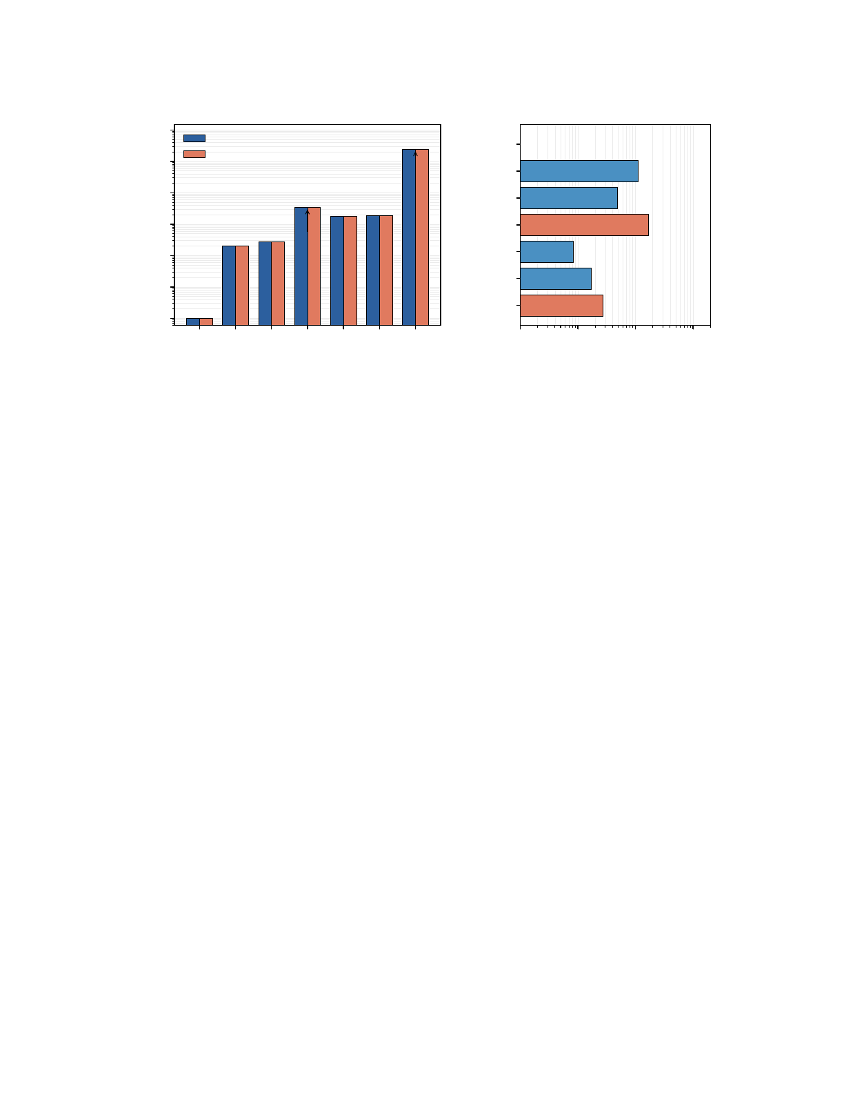
e
μ
π
±
τ
p
n
H
10
0
10
1
10
2
10
3
10
4
10
5
10
6
Mass ratio m
x
/m
e
(log scale)
new
new
(a) Predicted vs experimental mass ratios
Predicted C
x
Experimental m
x
/m
e
10
−3
10
−2
10
−1
10
0
|deviation| (%)
e
μ
π
±
τ
p
n
H
exact
0.11%
0.048%
0.17%
0.0083%
0.017%
0.027%
(b) Deviation from experiment
Figure 5: (a) Predicted topological costs
𝐶
𝑥
versus experimental mass ratios
𝑚
𝑥
/𝑚
𝑒
for the seven mass-bearing
particles on a log scale. The tauon at
𝐶
𝜏
= 3483
and the Higgs at
𝐶
𝐻
= 𝐾
2
3
(𝐾
𝐷
3
−𝐷
𝐷
) = 244,944
are the two new
predictions of this work; the other five are inherited from Part I [
1
]. (b) Absolute deviation
|𝑚
exp
−𝐶
𝑥
|/𝑚
exp
in
percent on a log scale. The electron is exact by definition. Five of the seven particles agree to better than
0.12 %
;
the tauon is the largest deviation at 0.17 %; the Higgs agrees within the PDG uncertainty on 𝑚
𝐻
.
15.2. Quantities not predicted
The framework does not yet fix the absolute neutrino mass scale, the individual quark masses, the numerical
CKM and PMNS entries, or the W and Z masses to percent precision. These are open construction problems
within the framework rather than failures of principle. Some require additional finite enumeration: the
masses require extending the f-vector formalism to a specific sub-structure (second-shell hadrons, twisted
worldsheets for the electroweak gauge bosons). CKM and PMNS additionally require an off-diagonal
dynamical mechanism coupling the triality sectors, which the framework does not contain. We list them as
concrete problems in Section 16.
15.3. Statistical significance of the mass matches
Integer mass formulas invite the objection that with enough structural constants available, some product of
them will land near any target. We quantify this look-elsewhere effect directly. Define the achievable set as
every integer of the form
𝐸
𝑠
×𝐶
𝑠
+ 𝜅
, with
𝐸
𝑠
drawn from the edge counts of the framework’s sub-structures
{1, 4, 16, 36, 78, 96, 𝐾
2
3
}
,
𝐶
𝑠
from the stabilizer-count sums appearing in the f-vector arithmetic (now including
the
𝑇
-quotient count 45), and
𝜅
from the correction terms the axioms generate
{0, ±1, ±𝐷, ±𝐷
2
, ±𝐷
3
, ±𝐾
2
3
𝐷
3
}
.
This yields 668 distinct integers (script
06_statistics.py
[
4
]); the two new structural constants are charged
for by including them. For each particle, let
Δ
be the achieved absolute deviation of the paper’s prediction
from the experimental ratio,
𝑘
the number of achievable integers matching at least as well,
𝜌
the local density
of the achievable set within
±10%
of the target, and
𝜆 = 2𝜌Δ
the expected number of chance matches of the
achieved quality under a uniform-density null. The chance probability of at least one match this good is
𝑝 = 1 − 𝑒
−𝜆
.
Three conclusions follow. The tauon match carries limited weight on its own: it is the unique achievable
integer in its window (
𝑘 = 1
), but the achievable set is dense enough near 3500 that a match of this quality
arises by chance with probability about
0.35
; its evidential contribution rests on the derivation of its existence
34

Table 8: Look-elsewhere analysis of the six predicted mass ratios (the electron is the normalization and is
excluded).
𝑘 = 1
means the paper’s prediction is the unique achievable integer matching that well.
∗
The Higgs row
is reported but excluded from the joint figure. Its subtraction grammar is fixed by Axiom 4, but the
𝐾
2
3
multiplier
rests on H5, which was introduced for this condensate; the row is excluded conservatively (see the caveats below).
Particle Δ 𝑘 𝜌 (per unit) 𝜆 𝑝
Muon 0.23 1 0.484 0.224 0.201
Pion 0.13 1 0.293 0.077 0.074
Tauon 5.77 1 0.037 0.431 0.350
Proton 0.15 1 0.071 0.022 0.021
Neutron 0.32 1 0.071 0.045 0.044
Higgs
∗
66.0 1 0.0002 0.030 0.029
and generation index and on the uniformity of the counting rule, not on the precision of its mass. The muon,
pion, proton, neutron and Higgs predictions are each the unique achievable integer matching as well as
observed, with individual chance probabilities between
0.02
and
0.20
. An independence approximation over
all six rows would give
1.4 × 10
−7
, or
1.5 × 10
−6
over the broad space of 1298 values; we report these for
completeness and do not rely on them.
Three caveats bound the joint figure, and we do not quote it in the abstract or conclusions. The proton
and neutron are not independent trials (
𝐶
𝑛
= 𝐶
𝑝
+ 𝐷
); treating them as one raises the joint probability by
about a factor of 20. The Higgs subtraction grammar is not free, since Axiom 4 mandates
𝐷
𝐷
for a volume
defect as it mandates
𝐷
2
for the muon, and with the
𝐾
2
3
resolution of H5 it leaves
𝐶
𝐻
= 𝐾
2
3
(𝐾
𝐷
3
− 𝐷
𝐷
)
as the
only expression in the inventory within
3𝜎
of the measured ratio; but H5 itself was introduced to evaluate
this condensate, so we exclude the Higgs row conservatively. With both adjustments the narrow-space joint
probability is roughly
1 × 10
−4
, the tauon contributing little. More fundamentally, the null model conditions
on the formula grammar as given and does not charge for the freedom exercised in constructing it: the lattice,
the polytopes, the arithmetic operations, the correction terms, and the allocation of formulas to particles. The
true look-elsewhere space includes model construction and is not enumerable, so the joint figure is not a
conventional significance and is not presented as one. What the table establishes is narrower: within the
framework’s own grammar, five of the six predictions are the unique achievable integers matching as well as
observed, and the tauon match is individually unremarkable and identified as such.
15.4. Limitations
Beyond the quantities not predicted, the framework carries the following limitations. Each is stated once here;
the open problems of Section 16 are the calculations that would remove them.
The mass identification itself. Rest mass as fault-tolerant verification cost is an interpretive postulate
inherited from Part I. This paper extends its reach and internal consistency; it does not derive the Landauer–
Einstein formula.
H1: the signature. The Lorentzian signature of
𝑥
0
is imposed, not obtained from the code. The
arrow condensate needs a gauge-invariant characterization (Elitzur’s theorem forbids a nonvanishing gauge-
noninvariant local order parameter). Lorentzian dynamics, the sign structure
𝐴(𝜕
𝑡
𝜙)
2
− 𝐵|∇𝜙|
2
, does not
follow from assigning a signature to bonds. Fourth-order isotropy of the slice is conditional on equal null and
spacelike hop weights, 𝑤 = 1 (Section 3.4).
H3 and the depth-3 exponent: the tauon. The count of Eq.
(7)
uses the muon’s conventions and adds two
elements that act trivially on any purely spatial defect, the time-reversal identification and the
𝐷
3
shedding.
35

Both are asserted from the structure of extraction rather than derived from the code; Table 6 records what
each does. The residual of
0.17 %
lies within the Part I accuracy band, and the chance probability of a match
at this level is about one in three (Section 15.3).
H5: the Higgs. The derivation of Section 12.1 rests on the nearest-reference measurement model, under
which a link degree of freedom resolves at
𝐾
3
levels rather than
2
𝐾
3
. The subtraction structure and the values
of 𝐾
3
and 𝐷 are anchored independently; the measurement-model lemma is not.
The sector rule and the sieve. The worldline sector rule of Section 7.1 is a consistency result across
seven assignments, not a derivation. Rule R4’s asymmetry between the confined 2-sheet and 3-sheet is
inherited from Part I; the
𝜋
0
is excluded by a scope argument (flavor superposition) rather than an axiom; the
cross-section axis of the sieve rests on classification by support dimension and sheet structure.
Scale separation. The emergent-symmetry arguments of Section 3.4 apply to long-wavelength modes,
𝑘𝑎 ≪ 1
; the defects that carry the masses are lattice-scale,
𝑘𝑎 ∼ 1
. Nothing established about the continuum
limit transfers automatically to them.
Verification scale. All
𝐷
4
computations are at
𝐿 = 4
(the
𝐷
3
VP code at
𝐿 = 6
). The parameters
𝑘 = 5𝐿
4
+ 2
and
𝑑 = 3
are confirmed there; the rate
𝑘/𝑛 → 5/6
is an extrapolation. The distance is not: it is
pinned at 3 by the triangles at every 𝐿.
15.5. Falsifiability
The framework forecloses two kinds of discoveries explicitly, the first conditional on H2a. A fourth-generation
charged lepton or quark would require a fourth admissible transverse worldline structure, and the constructed
three-level engagement ladder has no fourth rung; the exclusion is conditional because exhaustion at that level
is precisely hypothesis H2a (Section 6.2). A stable particle below the topological floor in the spatial sector
(i.e., a non-neutrino with
0 < 𝑚
𝑥
< 𝑚
𝑒
) would also falsify the model, since the electron is by construction the
minimum spatial defect. No such particle has been observed at the Large Hadron Collider (LHC) or anywhere
else [15].
15.6. Computational verification
Every numerical claim in this paper is reproduced by a verification suite of twenty-one scripts [
4
], executed
by
d4_run_all.py
in about four minutes on a standard laptop. Appendix A maps each script to the claims it
verifies and the section that makes them.
16. Open Problems
Most of the following are finite calculations within the framework; where an item instead requires a mechanism
the framework does not yet contain, we say so. They are grouped by the limitation they address.
H1. Derive the signature of
𝑥
0
from the code rather than imposing it; characterize the arrow condensate
gauge-invariantly; obtain the Lorentzian sign structure of the effective action; and derive
𝑤 = 1
. The
checkerboard structure of Section 3.2 is the natural place to look:
𝑤 = 1
is the statement that a site-to-void
hop costs the same in and out of a slice. Beyond that, connecting the lattice to continuum spacetime symmetry
needs a renormalization-group procedure and an assessment of the radiative fine-tuning problem of Ref. [
9
]
in this construction; we claim neither.
36

H3 and the depth-3 object. Exhibit, within the code, that a circuit running forward in
𝑥
0
cannot independently
record the syndrome of a future-directed object and its
𝑇
-image, or exhibit a circuit that can; either settles the
tauon count. Separately, enumerate the depth-3 tube of one proper-time step, two spatial cuboctahedra joined
by the null bonds, and compare its count with the
𝑇
-quotient of the full causal diamond; the
0.17 %
residual
is what that would explain or move.
H5. Select the nearest-reference measurement model from the verification axioms or from an information-
theoretic optimality principle. The rule’s dimension-portability prediction,
6
2
(6
2
− 2
2
) = 1152
for a
(2+1)-dimensional vacuum, is an internal consistency target.
The generation sector (H2a–c). An exhaustion argument for the engagement ladder; a mechanism that
breaks the axis-permutation symmetry and correlates transverse structure with depth (the Yukawa hierarchy
in a different vocabulary); an explicit construction of the quotient identifying the electron’s three anchorings
(H2c); and the physical identification of the three spatial winding classes of
𝐻
1
(𝑇
4
)
. Establishing or refuting
the identification of the coordinate 3-cycle with the outer-automorphism triality of Spin(8) belongs here.
The sector rule. Two calculations would promote it to a derivation: the mutual-information saturation of
Section 7.1, and a derivation of the electron’s residual
𝐶
𝑠
= 1
as an existence bit. A connecting argument for
rule R4’s asymmetry belongs to the same program, as does a defect-level treatment of flavor superpositions,
which would give the 𝜋
0
/𝜋
±
splitting.
Sectors not computed. The W and Z masses (
𝑚
𝑊
/𝑚
𝑒
≈ 1.575 × 10
5
,
𝑚
𝑍
/𝑚
𝑒
≈ 1.785 × 10
5
,
𝑚
𝑊
/𝑚
𝑍
≈
0.882 = cos 𝜃
𝑊
), from the 2-cell stabilizer overlaps of twisted worldsheets on the 24-cell skeleton with the
appropriate shedding for 2D extended states, once the cost functional is extended beyond compact footprints
(gauge sector, below); the second-shell hadrons
𝐾
,
Λ
,
Σ
,
𝐷
,
𝐵
, by the enumeration of Part I’s Section 6 at
the second shell; and the neutrino mass scale, which in the checkerboard reading is the verification cost
per reversal of a null worldline times its reversal rate, the second computable from the null-link condensate
density and the lattice spacing.
PMNS and CKM angles. These are a different problem from the masses, and it is worth saying why. The
verification cost assigns each generation a number, the eigenvalues of the mass matrix. A mixing angle is not
a property of eigenvalues: it measures the misalignment between the mass eigenbasis and the weak basis
and lives entirely in the off-diagonal entries, which the counting never produces: each defect is enumerated
independently and nothing relates one generation’s support to another’s. A derivation needs a mechanism that
couples the triality sectors rather than labeling them, and the framework does not contain one.
The gauge sector. The worldsheet correspondence of Section 10 places a continuous SU(2)×U(1) bundle
over a discrete polytope; replacing the bundle by a fiber polytope would keep the construction discrete
throughout, and whether the boson count survives is open. For color, the non-abelian link phases on the
hexagon loops and their coupling are open, as is the relation between the separation potential of Ref. [
3
] and
the code: Definition 1 fixes no verification cost for an extended object (Section 10.2), and an extension of
the cost functional beyond compact footprints, if one exists, would be where the metric-wall tension and the
sector rule that prices the confined state meet.
37

Code structure. Partition all 1282 logical qubits at
𝐿 = 4
by cellular dimension class and triality orbit,
completing the orbit structure of Section 6.3. Verify
𝑘 = 5𝐿
4
+2
at
𝐿 = 6, 8
to test the approach to
𝑘/𝑛 → 5/6
.
Determine which self-orthogonal subsets of the triangular plaquettes can be added as stabilizers to raise the
distance while retaining a high rate; adding all of them collapses
𝑘
to the Betti numbers (Section 4.2), so the
useful constructions lie strictly between. Whether a useful CSS code exists on the
𝐺
2
root lattice is open, and
the design strength of the shell (3 for
𝐷
3
, 5 for
𝐷
4
, 7 for
𝐸
8
) is a lattice invariant that could select among
substrates.
17. Conclusions
Reading one coordinate of the
𝐷
4
lattice as Lorentzian time makes the lattice the
𝐷
3
code time-stepped
along null bonds, with the two stabilizer types exchanging the
𝐷
3
sites and their voids at every step. On that
structure, with the five hypotheses of Section 2 stated in advance, the Part I framework reaches what it could
not reach in three dimensions.
Rigorous and verified: the vertex–plaquette code carries the Part I sector counts as literal stabilizer
content; its homological ladder realizes the Betti numbers
(4, 6, 4, 1)
of
𝑇
4
; the
𝐷
4
code has parameters
[[1536, 1282, 3]]
with weight-24 stabilizers; time reversal is a code automorphism fixing the spatial sub-
complex; color charge is paired on the code by a parity theorem; and the null bonds supply the coordinate-axis
directions the
𝐷
3
shell lacks, so that fourth-order isotropy of the slice holds when null and spacelike hops
carry equal weight. The sector assignments, underivable from spatial footprints alone (the muon and proton
share one), are reproduced by the worldline sector rule, and the sieve built on that rule yields 22 survivors
from 48 candidates, matching the Standard Model field-content count at the first shell.
Conditional and stated as such: the tauon at
78 × 45 − 27 = 3483
(
0.17 %
), by the muon’s counting rule
applied to the causal diamond modulo
𝑇
with depth-3 shedding, conditional on H3 and the exponent; the
Higgs at
𝐾
2
3
(𝐾
𝐷
3
− 𝐷
𝐷
) = 244,944
, within experimental uncertainty, conditional on H5; three generations,
conditional on H2a. Proposed and qualitative: neutrinos as null zigzags with mass set by their reversal rate;
the photon on the null links; confinement entering the cost only through the sector rule, with the separation
potential derived in the geometry of Ref. [3].
No parameter is fitted anywhere in the mass spectrum, no measured value enters any derivation, and every
choice is recorded in Table 5. What the framework does not do is listed in Section 15.4, and what would
remove each limitation in Section 16.
CRediT authorship contribution statement. Raghu Kulkarni: Writing – review & editing, Writing –
original draft, Visualization, Validation, Methodology, Conceptualization.
Declaration of competing interest. The author declares no known competing financial interests or personal
relationships that could have influenced the work reported in this paper.
Data availability. The complete verification suite described in Section 15.6 is archived with a persistent
identifier at doi:10.5281/zenodo.22393024 (Ref. [
4
]): twenty-one verification scripts, the master runner
d4_run_all.py
, the figure generators, and a README mapping each script to the claim it verifies. Running
d4_run_all.py
executes all twenty-one in about four minutes and reports pass or fail for each; the suite
requires
numpy
,
scipy
and
sympy
, with
matplotlib
for the figure generators. A working mirror is kept
at
github.com/raghu91302/ssmtheory/blob/main/d4_extended_scripts_v5.zip
. An interactive
38

3D visualization of the
𝐷
4
lattice and its 24-cell is hosted at
raghu91302.github.io/ssmtheory/d4_
interactive.html.
A. Verification scripts
The scripts below form the archived suite of Ref. [4].
script section verifies
01_structure_tensor.py 3 𝑆
𝜇𝜈
= 12𝛿
𝜇𝜈
exactly; the third moment
𝑇
𝜇𝜈𝜆
=
Í
𝑗
𝑛
𝜇
𝑗
𝑛
𝜈
𝑗
𝑛
𝜆
𝑗
vanishes by
centrosymmetry; emergence of the 𝐷
3
sub-lattice under the foliation.
02_24cell_triality.py 6 and 8
the 24-cell f-vector
(24, 96, 96, 24)
; the
8 +8 +8
triality split into three inscribed
16-cells; the 4–4–4 split of the 12
𝐷
3
spatial bonds across triality sets; the 72
raw squares (their
𝑇
-quotient to 45 and inversion quotient to 36 are computed in
script 20).
03_d4_css_code.py 3
full construction of the CSS code at
𝐿 = 4
, verifying
𝑛 = 1536
, uniform stabilizer
weight 24,
𝐻
𝑋
𝐻
𝑇
𝑍
= 0 (mod 2)
,
𝑘 = 5𝐿
4
+ 2 = 1282
, and
𝑑 ≥ 3
by exhaustive
weight-≤ 2 elimination on both sides.
04_mass_spectrum.py 15
all seven rest-mass and Higgs formulas, including the tauon
78 × 45 − 27 = 3483
and the structural identity
𝐶
𝐻
= 𝐾
2
3
(𝐾
𝐷
3
− 𝐷
𝐷
) = 244,944
, and their deviations
from experiment.
05_triality_code_
automorphism.py
6.3 and
12.1
the coordinate 3-cycle
𝜋
as a code automorphism; the orbit structure on the
1536 qubits (512 orbits of size 3, none fixed); explicit construction of three
triality-inequivalent worldline logical Z operators.
06_statistics.py 15.3
the achievable-integer spaces (523 narrow, 1048 broad), the per-particle window
densities and 𝜆 values of Table 8, and the joint chance probabilities.
07_sector_map.py 7.1
the muon–proton footprint degeneracy (identical 36-edge, 12-odd-vertex boundary
structure) and the reproduction of all seven sector assignments by the worldline
sector rule.
08_logical_
classification.py
4.2
the complete census of the
𝐷
4
code’s 1282 logical classes; every class reduces to
weight ≤ 9.
09_code_functional_
validation.py
4.1
the
𝐷
3
vertex–plaquette code
[[648, 3]]
and the exact reproduction of the sector
counts 17, 6, and 51 as cell-count functionals.
10_d4_plaquette_
code.py
4.2
the
𝐷
4
edge code
[[1536, 4]]
, the four weight-4 worldline logicals, and the
volume-scale membrane class.
11_face_qubit_code.py 4.2 the face-qubit code and the six coordinate worldsheet logicals.
12_complete_cells.py 4.2 the completed 3-cell inventory and the collapse to 𝑘 = 6 = dim 𝐻
2
(𝑇
4
).
13_top_rungs.py 4.2
the codes
[[3072, 4]]
and
[[384, 1]]
, the fundamental class, the honeycomb
incidence structure, and the factor-seven analysis.
14_rule_space_scan.py 12.1
the exhaustive scan of binary subtraction rules (37,334 values, maximum
167,281
)
and the vertex-figure verification (24, 96, 96, 24).
15_spherical_design.py 3.4
symbolic computation of the bond-set moments; the
𝐷
3
shell is a spherical
3-design with
𝑀
4
= 3(𝑘
2
)
2
−
Í
𝑖
𝑘
4
𝑖
, the
𝐷
4
shell a spherical 5-design with
𝑀
4
= 3(𝑘
2
)
2
exactly; and the measured anisotropy exponents
2.00
and
4.00
from
the exact lattice dispersion.
16_distance_exact.py 3.2
all 4096 triangles of the
𝐷
4
lattice at
𝐿 = 4
(and all 256 of
𝐷
3
) are weight-3
logical operators, closing the distance from above and giving
𝑑 = 3
exactly for
both codes.
17_photon_
sublattice.py
10
the
⟨100⟩
node–void sublattice is simple cubic and bipartite; the Hodge ranks of
its one-form sector at
𝐿 = 4
and
𝐿 = 6
(one pure-gauge and two transverse modes
per site, harmonic dimension
3 = 𝑏
1
(𝑇
3
)
); disjointness of the
⟨100⟩
links from
the code qubits; and the vanishing rank-three moment of the centrosymmetric
bond star.
39

script section verifies
18_matter_coupling.py 10
every
⟨110⟩
edge is covered by exactly two two-step
⟨100⟩
paths through an
octahedral void, and the two paths differ by one cubic plaquette.
19_gluon_
confinement.py
10
24 odd cycles through each site of the
⟨110⟩
shell, failure of two-coloring, and
the fact that every one of the twelve bonds lies on an odd cycle.
20_lorentzian_
signature.py
3.4, 3.2,
3.3, 8 and
14
the checkerboard slicing of Z- and X-sites at
𝐿 = 4
; the
12 + 12
spacelike/null
split of the bonds and the
48 + 48
split of the shell edges with no future–past
edge; time reversal
𝑇
as a code automorphism fixing the spatial sub-complex; the
𝑇
-orbit counts
60/18/45
on the 24-cell against
48/12/36
under inversion; the
tauon count
78 ×45 −27 = 3483
with every row of Table 6; and the spatial fourth
moment 3|k|
4
+ (𝑤 − 1)
Í
𝑖
𝑘
4
𝑖
.
21_color_kinematics.py 10
the parity theorem on the
𝐷
3
code (
𝐻
𝑍
and
𝐻
𝑋
column weights 2; all 4095
hexagon Pauli operators even, none single-vertex-charged); and the hexagon link
template (two routes of weight 3, each disturbing six void checks, loop outside
the 𝑋-stabilizer group, pairwise overlap, composition to the alternating triple).
References
[1]
R. Kulkarni, The Mass–Energy–Information Equivalence: A bottom-up identification of the particle spectrum via
FCC lattice error correction, Phys. Open 27 (2026) 100414. doi.org/10.1016/j.physo.2026.100414
[2]
R. Kulkarni, A 67%-rate CSS code on the FCC lattice:
[[192, 130, 3]]
from weight-12 stabilizers,
arXiv:2603.20294 (2026). arxiv.org/abs/2603.20294
[3]
R. Kulkarni, Matter as incomplete crystallization: quark charges, color confinement, and the proton mass from a
single extra node in the vacuum lattice, Phys. Open 27, 100423 (2026). doi:10.1016/j.physo.2026.100423.
[4]
R. Kulkarni, Verification suite for the
𝐷
4
extended mass–energy–information framework, Zenodo (2026),
doi:10.5281/zenodo.22393024. Twenty-one scripts, master runner
d4_run_all.py
, figure generators, and a
README mapping each script to the claim it verifies. Mirrored at
github.com/raghu91302/ssmtheory/
blob/main/d4_extended_scripts_v5.zip.
[5]
J. H. Conway and N. J. A. Sloane, Sphere Packings, Lattices and Groups, Springer, 3rd ed., 1999. Chapters 4 (the
𝐷
𝑛
family) and 7 (the 24-cell). doi.org/10.1007/978-1-4757-6568-7
[6]
D. A. Huse, W. Krauth, R. Moessner and S. L. Sondhi, Coulomb and liquid dimer models in three dimensions,
Phys. Rev. Lett. 91, 167004 (2003). doi:10.1103/PhysRevLett.91.167004.
[7]
C. L. Henley, The Coulomb phase in frustrated systems, Annu. Rev. Condens. Matter Phys. 1, 179 (2010).
doi:10.1146/annurev-conmatphys-070909-104138.
[8]
P. Delsarte, J. M. Goethals and J. J. Seidel, Spherical codes and designs, Geom. Dedicata 6 (1977) 363.
doi.org/10.1007/BF03187604
[9]
J. Collins, A. Pérez, D. Sudarsky, L. Urrutia and H. Vucetich, Lorentz invariance and quantum gravity: an additional
fine-tuning problem?, Phys. Rev. Lett. 93 (2004) 191301. doi.org/10.1103/PhysRevLett.93.191301
[10]
S. Liberati and L. Maccione, Lorentz violation: motivation and new constraints, Ann. Rev. Nucl. Part. Sci. 59
(2009) 245. doi.org/10.1146/annurev.nucl.010909.083640
[11]
T. C. Hales, A proof of the Kepler conjecture, Ann. Math. 162 (2005) 1065.
doi.org/10.4007/annals.2005.
162.1065
[12]
J. F. Adams, Lectures on Exceptional Lie Groups, Chicago Lectures in Mathematics, University of Chicago Press,
1996. ISBN 978-0-226-00527-0. search.worldcat.org/isbn/9780226005270
40

[13]
ALEPH, DELPHI, L3, OPAL, SLD Collaborations, Precision electroweak measurements on the Z resonance,
Phys. Rep. 427 (2006) 257. doi.org/10.1016/j.physrep.2005.12.006
[14]
E. Tiesinga et al., CODATA recommended values of the fundamental physical constants: 2022, Rev. Mod. Phys.
97 (2024) 025002. doi.org/10.1103/RevModPhys.97.025002
[15]
R. L. Workman et al. (Particle Data Group), Review of Particle Physics, Prog. Theor. Exp. Phys. (2022) 083C01.
doi.org/10.1093/ptep/ptac097
[16] K. G. Wilson, Confinement of quarks, Phys. Rev. D 10 (1974) 2445. doi.org/10.1103/PhysRevD.10.2445
[17]
R. Landauer, Irreversibility and heat generation in the computing process, IBM J. Res. Dev. 5 (1961) 183.
doi.org/10.1147/rd.53.0183
41
