Gauge Theory on the
D
4
Root Lattice:
A Single-Coupling Triangular Action with
F
4
-Protected
O(a
2
)
Rotational Improvement
Raghu Kulkarni
*
SSMTheory Group, IDrive Inc., Calabasas, CA 91302, USA
2026
Abstract
We study
SU (N)
Wilson lattice gauge theory on the
D
4
root lattice, the densest sphere pack-
ing in four dimensions and the lattice with the maximum kissing number
K = 24
in
R
4
.
D
4
is a
natural non-hypercubic discretization of four-dimensional Euclidean spacetime: its coordination
polytope is the self-dual
24
-cell (Weyl group
F
4
, order
1152
), and every integer slice
x
4
=
const
is a three-dimensional face-centred cubic (FCC) lattice. Because the
24
-cell has only triangular
faces, the Wilson gauge action is single-coupling, with
12
unoriented links and
32
triangular
plaquettes per cell. We report a chain of explicit results for this action. (i) The plaquette
stiness tensor is exactly
T
µνρσ
∝ (δ
µρ
δ
νσ
− δ
µσ
δ
νρ
)
, so the leading continuum
Tr(F
µν
F
µν
)
term is isotropic and the
O(a
2
)
gauge anisotropy present in the hypercubic discretization is
absent. (ii) The tree-level coupling is xed,
g
2
eff
= N/β
on
D
4
against
2N/β
on the hypercubic
lattice. (iii) The tree-level free gauge dispersion is rotationally isotropic through
O(k
4
)
: its di-
rectional anisotropy scales as
|k|
4
, against
|k|
2
for the unimproved hypercubic Wilson action, so
D
4
realizes automatic, untuned, single-coupling tree-level
O(a
2
)
rotational improvement of the
gauge action. (iv) The absence of the
O(a
2
)
rotational-anisotropy counterterm is protected to
all orders in perturbation theory by the
F
4
point group, whose quartic invariant spaceunlike
the hypercubic
B
4
contains no anisotropic invariant, so this counterterm is never generated.
We are explicit about what is
not
xed: the one-loop
Λ
lat
/Λ
MS
ratio and the (symmetry-
allowed, isotropic)
O(a
2
)
artifact coecient, the magnitude of the
O(a
4
)
corrections, and the
computational-cost comparison remain open. The naive and Wilson
fermion
sector on
D
4
the
Dirac-operator factorization, the doubler classication, and the geometric Wilson massesis
treated in a companion paper [11]. All numerical claims are reproduced by a public verication
bundle.
1 Introduction
Lattice QCD is almost universally formulated on the hypercubic lattice
Z
4
[4], for the practical
reasons that it is simple to reason about and simple to implement. It is not, however, the only four-
dimensional lattice available, and the question of whether a more isotropic substrate reduces dis-
cretization error is an old one. The same motivation drives the Symanzik improvement program [5]
and the perfect-/xed-point-action program [6]: the hypercubic action breaks the Euclidean rota-
tion group
SO(4)
to the cubic subgroup already at
O(a
2
)
, and a lattice with a larger automorphism
group postpones or removes the leading anisotropic operator.
*
raghu@idrive.com
1
Non-hypercubic lattice gauge theory is a small but established literature. Celmaster studied
gauge elds on the body-centred hypercubic lattice [8]; the
D
4
lattice in particular has long been
noted as a more symmetric four-dimensional alternative (see e.g. the pedagogical discussion in [9]),
generally set aside because the practical costs were judged to outweigh the isotropy gain. The present
paper revisits the gauge sector of this option: it works out the explicit single-coupling triangular
Wilson action on
D
4
, its continuum limit, and its dispersion, and shows that the absence of
O(a
2
)
rotational anisotropy is protected by the lattice point group to all orders. The companion fermion
sectorthe naive Dirac operator, doubler classication, and geometric Wilson masses on the FCC
and
D
4
latticesis developed separately [11]. No fermion-sector result is used in the gauge-sector
arguments below; the two papers share only the
D
4
geometry of Sections 23.
Scope and reading.
We adopt the standard interpretation throughout:
D
4
is a discretization of
continuum four-dimensional Euclidean spacetime, with the
a → 0
limit recovering continuum Yang
Mills. The results below are structural the per-cell Wilson data, the leading-order continuum
gauge action and its exact stiness tensor, the tree-level coupling and gauge dispersion, and the
point-group protection of the latter. They characterize the gauge formulation analytically; they do
not include the one-loop matching or the dynamical simulations that would establish a quantitative
advantage over
Z
4
, and we ag those as the natural next steps rather than claiming them here.
Why FCC and
D
4
are distinguished.
In three dimensions FCC is the densest packing (Hales [1]),
has the maximum kissing number
K = 12
for a Bravais lattice, and has isotropic structure tensor
S
FCC
µν
= 4δ
µν
. The four-dimensional analog with all three properties simultaneously densest
packing, maximum kissing number, isotropic structure tensor is
D
4
[2]. We note for honesty that
no
one
of these properties is unique to
D
4
among lattices containing FCC slices: the orthogonal
stack
FCC ⊕ aZ
also has FCC at every integer slice, but it is neither densest nor isotropic in its
temporal direction. It is the
conjunction
of the three properties that singles out
D
4
, and we do not
claim a uniqueness theorem beyond that.
Main results.
1.
Slicing
(Section 3).
D
4
∩{x
4
= 0} = FCC
, and the
24
nearest neighbors partition as
12 + 12
(twelve spatial, six forward, six backward).
2.
Wilson gauge action
(Section 4). Single coupling,
12
links and
32
triangular plaquettes per
unit cell; the
24
-cell has no square plaquettes.
3.
Leading-order isotropy
(Section 5). The plaquette stiness tensor is exactly proportional
to
(δ
µρ
δ
νσ
− δ
µσ
δ
νρ
)
, so the leading continuum
Tr(F
µν
F
µν
)
term is isotropic and the
O(a
2
)
rotational-anisotropy artifact is absent.
4.
Tree-level coupling
(Section 5.1).
g
2
eff
= N/β
on
D
4
, against
2N/β
on the hypercubic lattice.
5.
Gauge dispersion
(Section 5.2). The tree-level free dispersion is rotationally isotropic through
O(k
4
)
; its directional anisotropy scales as
|k|
4
, versus
|k|
2
for unimproved hypercubic Wilson.
6.
All-orders protection
(Section 5.3). The
F
4
point group admits no anisotropic quartic invari-
ant, so the
O(a
2
)
rotational-anisotropy counterterm is forbidden to all orders in perturbation
theory.
2
2 The
D
4
Root Lattice
D
4
is the index-2 even sublattice of
Z
4
,
D
4
=
(x
1
, x
2
, x
3
, x
4
) ∈ Z
4
: x
1
+ x
2
+ x
3
+ x
4
≡ 0 (mod 2)
,
(1)
equivalently the integer span of the simple roots
α
1
= e
1
−e
2
,
α
2
= e
2
−e
3
,
α
3
= e
3
−e
4
,
α
4
= e
3
+e
4
of
so(8)
. A fundamental cell has volume
2
.
2.1 Kissing set and structure tensor
The minimum norm is
√
2
, realized by
N(D
4
) = {±e
i
± e
j
: 1 ≤ i < j ≤ 4},
(2)
a set of
4
2
· 2
2
= 24
vectors, each with
|n|
2
= 2
. This is the kissing number of
D
4
and equals the
kissing number of
R
4
[2].
Proposition 1
(Isotropy of
D
4
)
.
S
µν
≡
P
n∈N (D
4
)
n
µ
n
ν
= 12 δ
µν
; with unit-length normalization
ˆn = n/
√
2
,
ˆ
S
µν
= 6 δ
µν
.
Proof.
For
µ = ν
the only contributing vectors are
±e
µ
± e
ν
, and
P
±±
(±1)(±1) = 0
. For xed
µ
,
the contributing vectors are
±e
µ
±e
ν
for the three
ν = µ
, i.e.
12
vectors each contributing
n
2
µ
= 1
,
so
S
µµ
= 12
. Index symmetry gives equality of the four diagonal entries. Unit normalization divides
by
|n|
2
= 2
.
This is the four-dimensional analog of
S
FCC
µν
= 4δ
µν
and guarantees that the leading discrete
kinetic action is
SO(4)
-invariant at
O(a
2
)
.
2.2 The 24-cell
The
24
kissing vectors are the vertices of a
24
-cell [3], the unique self-dual regular 4-polytope, with
V = 24
,
E = 96
,
F = 96
triangular faces,
C = 24
octahedral cells, and
V −E + F − C = 0
. Every
face is an equilateral triangle; there are no square faces. The symmetry group is the Weyl group
F
4
of order
1152
, containing the FCC point group
O
h
(order
48
) with index
1152/48 = 24
.
3 Slicing:
D
4
over FCC time-slices
Theorem 1
(Slicing)
.
D
4
∩ {x
4
= 0} = FCC
, where
FCC = {(x
1
, x
2
, x
3
) ∈ Z
3
: x
1
+ x
2
+ x
3
≡
0 (mod 2)}
.
Proof.
(x
1
, x
2
, x
3
, 0) ∈ D
4
i
x
1
+ x
2
+ x
3
≡ 0 (mod 2)
, which is the FCC condition. Even-
c
slices
x
4
= c
give FCC; odd-
c
slices give the shifted (odd-parity) FCC coset.
Proposition 2
(
12 + 12
decomposition)
.
N(D
4
) = N
spatial
⊔ N
+
temporal
⊔ N
−
temporal
, with
N
spatial
=
{±e
i
±e
j
: 1 ≤ i < j ≤ 3}
(
12
vectors, the FCC kissing set) and
N
±
temporal
= {±e
i
±e
4
: 1 ≤ i ≤ 3}
(
6
vectors each).
Proof.
Each
n = ±e
i
± e
j
. If
j < 4
then
n
4
= 0
(
3
2
· 4 = 12
); if
j = 4
then
n
4
= ±1
(
3 · 2 = 6
per
sign).
3
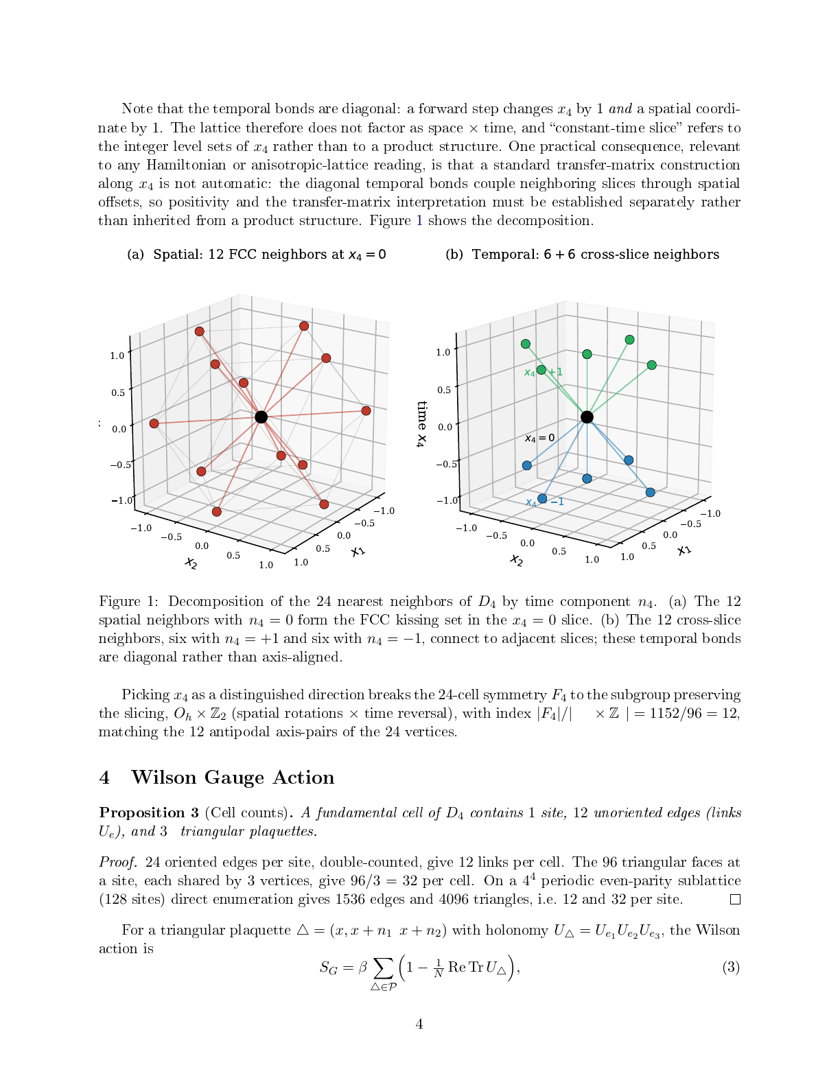
Note that the temporal bonds are diagonal: a forward step changes
x
4
by
1
and
a spatial coordi-
nate by
1
. The lattice therefore does not factor as space
×
time, and constant-time slice refers to
the integer level sets of
x
4
rather than to a product structure. One practical consequence, relevant
to any Hamiltonian or anisotropic-lattice reading, is that a standard transfer-matrix construction
along
x
4
is not automatic: the diagonal temporal bonds couple neighboring slices through spatial
osets, so positivity and the transfer-matrix interpretation must be established separately rather
than inherited from a product structure. Figure 1 shows the decomposition.
1.0
0.5
0.0
0.5
1.0
x
1
1.0
0.5
0.0
0.5
1.0
x
2
1.0
0.5
0.0
0.5
1.0
x
3
(a) Spatial: 12 FCC neighbors at
x
4
= 0
1.0
0.5
0.0
0.5
1.0
x
1
1.0
0.5
0.0
0.5
1.0
x
2
1.0
0.5
0.0
0.5
1.0
time
x
4
x
4
= +1
x
4
= 1
x
4
= 0
(b) Temporal:
6 + 6
cross-slice neighbors
Figure 1: Decomposition of the
24
nearest neighbors of
D
4
by time component
n
4
. (a) The
12
spatial neighbors with
n
4
= 0
form the FCC kissing set in the
x
4
= 0
slice. (b) The
12
cross-slice
neighbors, six with
n
4
= +1
and six with
n
4
= −1
, connect to adjacent slices; these temporal bonds
are diagonal rather than axis-aligned.
Picking
x
4
as a distinguished direction breaks the
24
-cell symmetry
F
4
to the subgroup preserving
the slicing,
O
h
×Z
2
(spatial rotations
×
time reversal), with index
|F
4
|/|O
h
×Z
2
| = 1152/96 = 12
,
matching the
12
antipodal axis-pairs of the
24
vertices.
4 Wilson Gauge Action
Proposition 3
(Cell counts)
.
A fundamental cell of
D
4
contains
1
site,
12
unoriented edges (links
U
e
), and
32
triangular plaquettes.
Proof.
24
oriented edges per site, double-counted, give
12
links per cell. The
96
triangular faces at
a site, each shared by
3
vertices, give
96/3 = 32
per cell. On a
4
4
periodic even-parity sublattice
(
128
sites) direct enumeration gives
1536
edges and
4096
triangles, i.e.
12
and
32
per site.
For a triangular plaquette
△ = (x, x + n
1
, x + n
2
)
with holonomy
U
△
= U
e
1
U
e
2
U
e
3
, the Wilson
action is
S
G
= β
X
△∈P
1 −
1
N
Re Tr U
△
,
(3)
4
with a single coupling
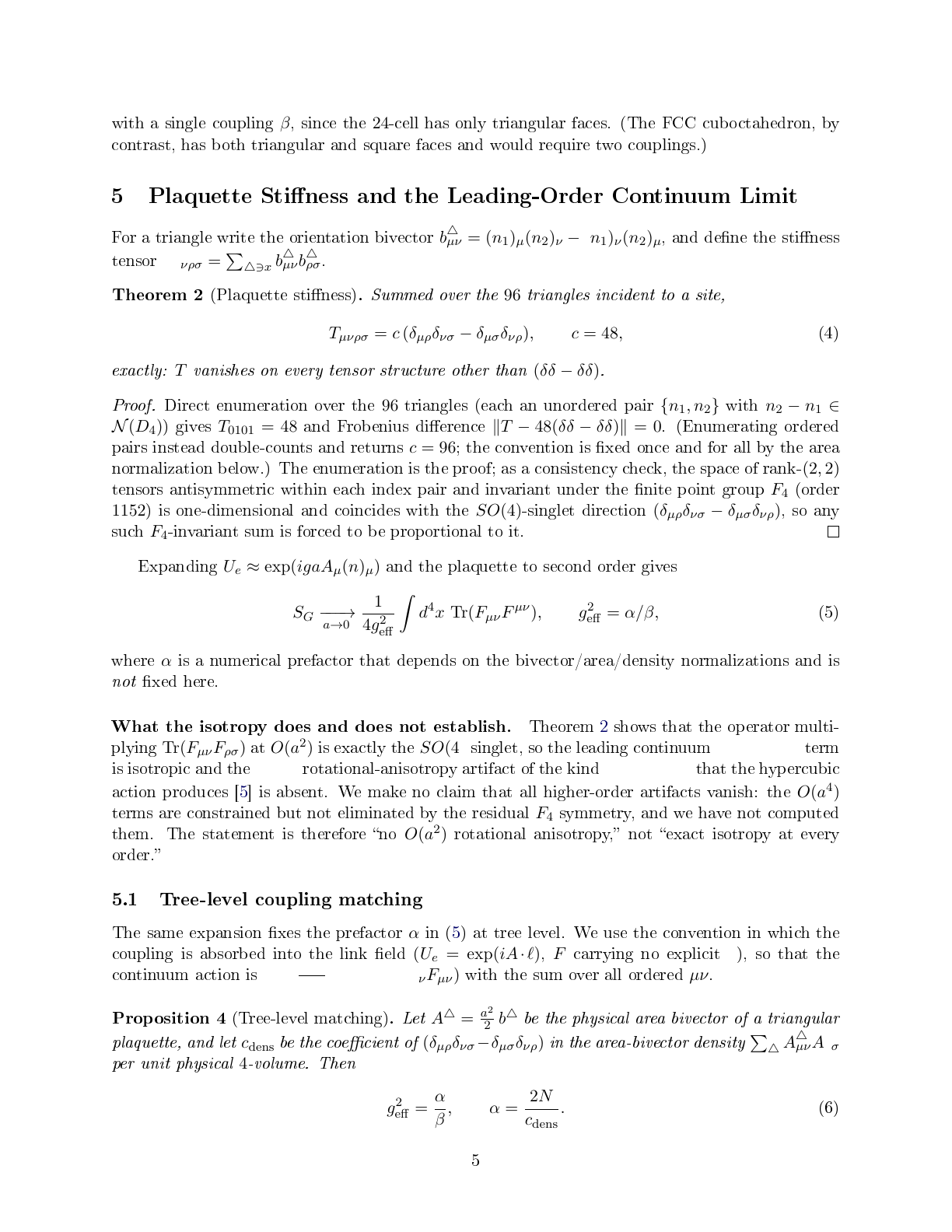
β
, since the
24
-cell has only triangular faces. (The FCC cuboctahedron, by
contrast, has both triangular and square faces and would require two couplings.)
5 Plaquette Stiness and the Leading-Order Continuum Limit
For a triangle write the orientation bivector
b
△
µν
= (n
1
)
µ
(n
2
)
ν
−(n
1
)
ν
(n
2
)
µ
, and dene the stiness
tensor
T
µνρσ
=
P
△∋x
b
△
µν
b
△
ρσ
.
Theorem 2
(Plaquette stiness)
.
Summed over the
96
triangles incident to a site,
T
µνρσ
= c (δ
µρ
δ
νσ
− δ
µσ
δ
νρ
), c = 48,
(4)
exactly:
T
vanishes on every tensor structure other than
(δδ − δδ)
.
Proof.
Direct enumeration over the
96
triangles (each an unordered pair
{n
1
, n
2
}
with
n
2
− n
1
∈
N(D
4
)
) gives
T
0101
= 48
and Frobenius dierence
∥T − 48(δδ − δδ)∥ = 0
. (Enumerating ordered
pairs instead double-counts and returns
c = 96
; the convention is xed once and for all by the area
normalization below.) The enumeration is the proof; as a consistency check, the space of rank-
(2, 2)
tensors antisymmetric within each index pair and invariant under the nite point group
F
4
(order
1152
) is one-dimensional and coincides with the
SO(4)
-singlet direction
(δ
µρ
δ
νσ
− δ
µσ
δ
νρ
)
, so any
such
F
4
-invariant sum is forced to be proportional to it.
Expanding
U
e
≈ exp(igaA
µ
(n)
µ
)
and the plaquette to second order gives
S
G
−−−→
a→0
1
4g
2
eff
Z
d
4
x Tr(F
µν
F
µν
), g
2
eff
= α/β,
(5)
where
α
is a numerical prefactor that depends on the bivector/area/density normalizations and is
not
xed here.
What the isotropy does and does not establish.
Theorem 2 shows that the operator multi-
plying
Tr(F
µν
F
ρσ
)
at
O(a
2
)
is exactly the
SO(4)
singlet, so the leading continuum
Tr(F
µν
F
µν
)
term
is isotropic and the
O(a
2
)
rotational-anisotropy artifact of the kind
P
µ
Tr(F
2
µν
)
that the hypercubic
action produces [5] is absent. We make no claim that all higher-order artifacts vanish: the
O(a
4
)
terms are constrained but not eliminated by the residual
F
4
symmetry, and we have not computed
them. The statement is therefore no
O(a
2
)
rotational anisotropy, not exact isotropy at every
order.
5.1 Tree-level coupling matching
The same expansion xes the prefactor
α
in (5) at tree level. We use the convention in which the
coupling is absorbed into the link eld (
U
e
= exp(iA·ℓ)
,
F
carrying no explicit
g
), so that the
continuum action is
S =
1
2g
2
eff
R
d
4
x Tr(F
µν
F
µν
)
with the sum over all ordered
µν
.
Proposition 4
(Tree-level matching)
.
Let
A
△
=
a
2
2
b
△
be the physical area bivector of a triangular
plaquette, and let
c
dens
be the coecient of
(δ
µρ
δ
νσ
−δ
µσ
δ
νρ
)
in the area-bivector density
P
△
A
△
µν
A
△
ρσ
per unit physical
4
-volume. Then
g
2
eff
=
α
β
, α =
2N
c
dens
.
(6)
5
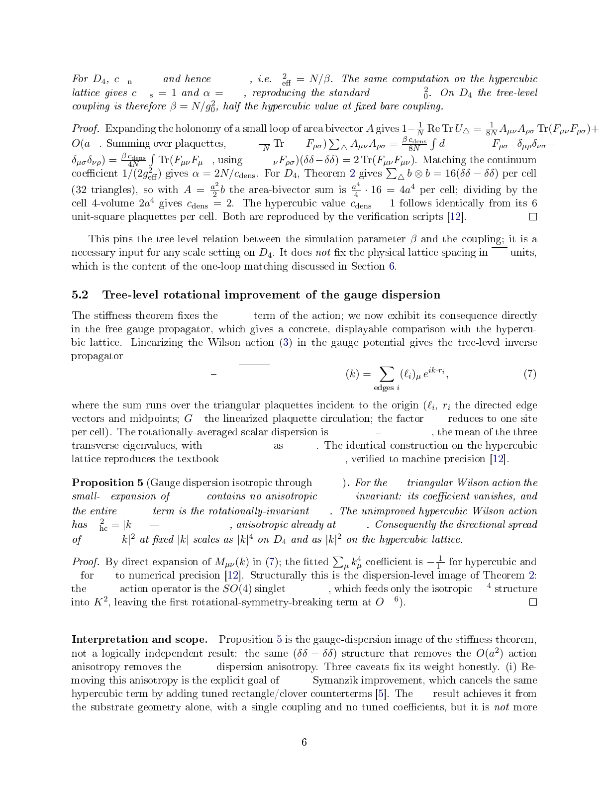
For
D
4
,
c
dens
= 2
and hence
α = N
, i.e.
g
2
eff
= N/β
. The same computation on the hypercubic
lattice gives
c
dens
= 1
and
α = 2N
, reproducing the standard
β = 2N/g
2
0
. On
D
4
the tree-level
coupling is therefore
β = N/g
2
0
, half the hypercubic value at xed bare coupling.
Proof.
Expanding the holonomy of a small loop of area bivector
A
gives
1−
1
N
Re Tr U
△
=
1
8N
A
µν
A
ρσ
Tr(F
µν
F
ρσ
)+
O(a
6
)
. Summing over plaquettes,
S
G
=
β
8N
Tr(F
µν
F
ρσ
)
P
△
A
µν
A
ρσ
=
β c
dens
8N
R
d
4
x Tr(F
µν
F
ρσ
)(δ
µρ
δ
νσ
−
δ
µσ
δ
νρ
) =
β c
dens
4N
R
Tr(F
µν
F
µν
)
, using
Tr(F
µν
F
ρσ
)(δδ−δδ) = 2 Tr(F
µν
F
µν
)
. Matching the continuum
coecient
1/(2g
2
eff
)
gives
α = 2N/c
dens
. For
D
4
, Theorem 2 gives
P
△
b ⊗ b = 16(δδ − δδ)
per cell
(
32
triangles), so with
A =
a
2
2
b
the area-bivector sum is
a
4
4
· 16 = 4a
4
per cell; dividing by the
cell
4
-volume
2a
4
gives
c
dens
= 2
. The hypercubic value
c
dens
= 1
follows identically from its
6
unit-square plaquettes per cell. Both are reproduced by the verication scripts [12].
This pins the tree-level relation between the simulation parameter
β
and the coupling; it is a
necessary input for any scale setting on
D
4
. It does
not
x the physical lattice spacing in
MS
units,
which is the content of the one-loop matching discussed in Section 6.
5.2 Tree-level rotational improvement of the gauge dispersion
The stiness theorem xes the
O(a
2
)
term of the action; we now exhibit its consequence directly
in the free gauge propagator, which gives a concrete, displayable comparison with the hypercu-
bic lattice. Linearizing the Wilson action (3) in the gauge potential gives the tree-level inverse
propagator
M
µν
(k) =
1
3
X
△∋0
G
△
µ
(k) G
△
ν
(k), G
△
µ
(k) =
X
edges
i
(ℓ
i
)
µ
e
ik·r
i
,
(7)
where the sum runs over the triangular plaquettes incident to the origin (
ℓ
i
,
r
i
the directed edge
vectors and midpoints;
G
△
the linearized plaquette circulation; the factor
1/3
reduces to one site
per cell). The rotationally-averaged scalar dispersion is
K
2
(k) ≡
1
3
Tr M
µν
(k)
, the mean of the three
transverse eigenvalues, with
K
2
(k) → |k|
2
as
k → 0
. The identical construction on the hypercubic
lattice reproduces the textbook
K
2
hc
(k) =
P
µ
4 sin
2
(k
µ
/2)
, veried to machine precision [12].
Proposition 5
(Gauge dispersion isotropic through
O(k
4
)
)
.
For the
D
4
triangular Wilson action the
small-
k
expansion of
K
2
(k)
contains no anisotropic
P
µ
k
4
µ
invariant: its coecient vanishes, and
the entire
O(k
4
)
term is the rotationally-invariant
|k|
4
. The unimproved hypercubic Wilson action
has
K
2
hc
= |k|
2
−
1
12
P
µ
k
4
µ
+O(k
6
)
, anisotropic already at
O(k
4
)
. Consequently the directional spread
of
K
2
(k)/|k|
2
at xed
|k|
scales as
|k|
4
on
D
4
and as
|k|
2
on the hypercubic lattice.
Proof.
By direct expansion of
M
µν
(k)
in (7); the tted
P
µ
k
4
µ
coecient is
−
1
12
for hypercubic and
0
for
D
4
to numerical precision [12]. Structurally this is the dispersion-level image of Theorem 2:
the
O(a
2
)
action operator is the
SO(4)
singlet
(δδ −δδ)
, which feeds only the isotropic
|k|
4
structure
into
K
2
, leaving the rst rotational-symmetry-breaking term at
O(k
6
)
.
Interpretation and scope.
Proposition 5 is the gauge-dispersion image of the stiness theorem,
not a logically independent result: the same
(δδ − δδ)
structure that removes the
O(a
2
)
action
anisotropy removes the
O(k
4
)
dispersion anisotropy. Three caveats x its weight honestly. (i) Re-
moving this anisotropy is the explicit goal of
O(a
2
)
Symanzik improvement, which cancels the same
hypercubic term by adding tuned rectangle/clover counterterms [5]. The
D
4
result achieves it from
the substrate geometry alone, with a single coupling and no tuned coecients, but it is
not
more
6
10
1
10
0
|
k
|
a
10
8
10
7
10
6
10
5
10
4
10
3
10
2
10
1
directional spread of
K
2
(
k
)/|
k
|
2
(a) Gauge-dispersion rotational anisotropy
hypercubic Wilson ( |
k
|
2
)
D
4
triangular ( |
k
|
4
)
axis
(1100)
diag (1111)
0.94
0.96
0.98
1.00
1.02
1.04
K
2
(
k
)/|
k
|
2
(norm. to mean)
(b) Direction dependence, |
k
|
a
= 1.4
hypercubic Wilson
D
4
triangular
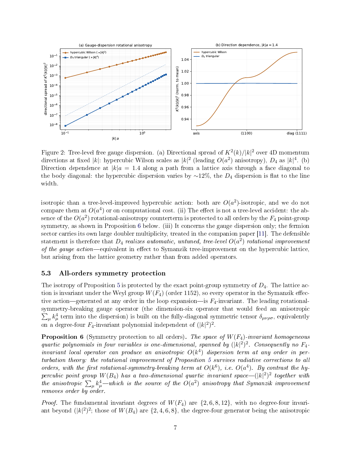
Figure 2: Tree-level free gauge dispersion. (a) Directional spread of
K
2
(k)/|k|
2
over
4
D momentum
directions at xed
|k|
: hypercubic Wilson scales as
|k|
2
(leading
O(a
2
)
anisotropy),
D
4
as
|k|
4
. (b)
Direction dependence at
|k|a = 1.4
along a path from a lattice axis through a face diagonal to
the body diagonal: the hypercubic dispersion varies by
∼12%
, the
D
4
dispersion is at to the line
width.
isotropic than a tree-level-improved hypercubic action: both are
O(a
2
)
-isotropic, and we do not
compare them at
O(a
4
)
or on computational cost. (ii) The eect is not a tree-level accident: the ab-
sence of the
O(a
2
)
rotational-anisotropy counterterm is protected to all orders by the
F
4
point-group
symmetry, as shown in Proposition 6 below. (iii) It concerns the gauge dispersion only; the fermion
sector carries its own large doubler multiplicity, treated in the companion paper [11]. The defensible
statement is therefore that
D
4
realizes automatic, untuned, tree-level
O(a
2
)
rotational improvement
of the gauge action
equivalent in eect to Symanzik tree-improvement on the hypercubic lattice,
but arising from the lattice geometry rather than from added operators.
5.3 All-orders symmetry protection
The isotropy of Proposition 5 is protected by the exact point-group symmetry of
D
4
. The lattice ac-
tion is invariant under the Weyl group
W (F
4
)
(order
1152
), so every operator in the Symanzik eec-
tive actiongenerated at any order in the loop expansionis
F
4
-invariant. The leading rotational-
symmetry-breaking gauge operator (the dimension-six operator that would feed an anisotropic
P
µ
k
4
µ
term into the dispersion) is built on the fully-diagonal symmetric tensor
δ
µνρσ
, equivalently
on a degree-four
F
4
-invariant polynomial independent of
(|k|
2
)
2
.
Proposition 6
(Symmetry protection to all orders)
.
The space of
W (F
4
)
-invariant homogeneous
quartic polynomials in four variables is one-dimensional, spanned by
(|k|
2
)
2
. Consequently no
F
4
-
invariant local operator can produce an anisotropic
O(k
4
)
dispersion term at any order in per-
turbation theory: the rotational improvement of Proposition 5 survives radiative corrections to all
orders, with the rst rotational-symmetry-breaking term at
O(k
6
)
, i.e.
O(a
4
)
. By contrast the hy-
percubic point group
W (B
4
)
has a two-dimensional quartic invariant space
(|k|
2
)
2
together with
the anisotropic
P
µ
k
4
µ
which is the source of the
O(a
2
)
anisotropy that Symanzik improvement
removes order by order.
Proof.
The fundamental invariant degrees of
W (F
4
)
are
{2, 6, 8, 12}
, with no degree-four invari-
ant beyond
(|k|
2
)
2
; those of
W (B
4
)
are
{2, 4, 6, 8}
, the degree-four generator being the anisotropic
7
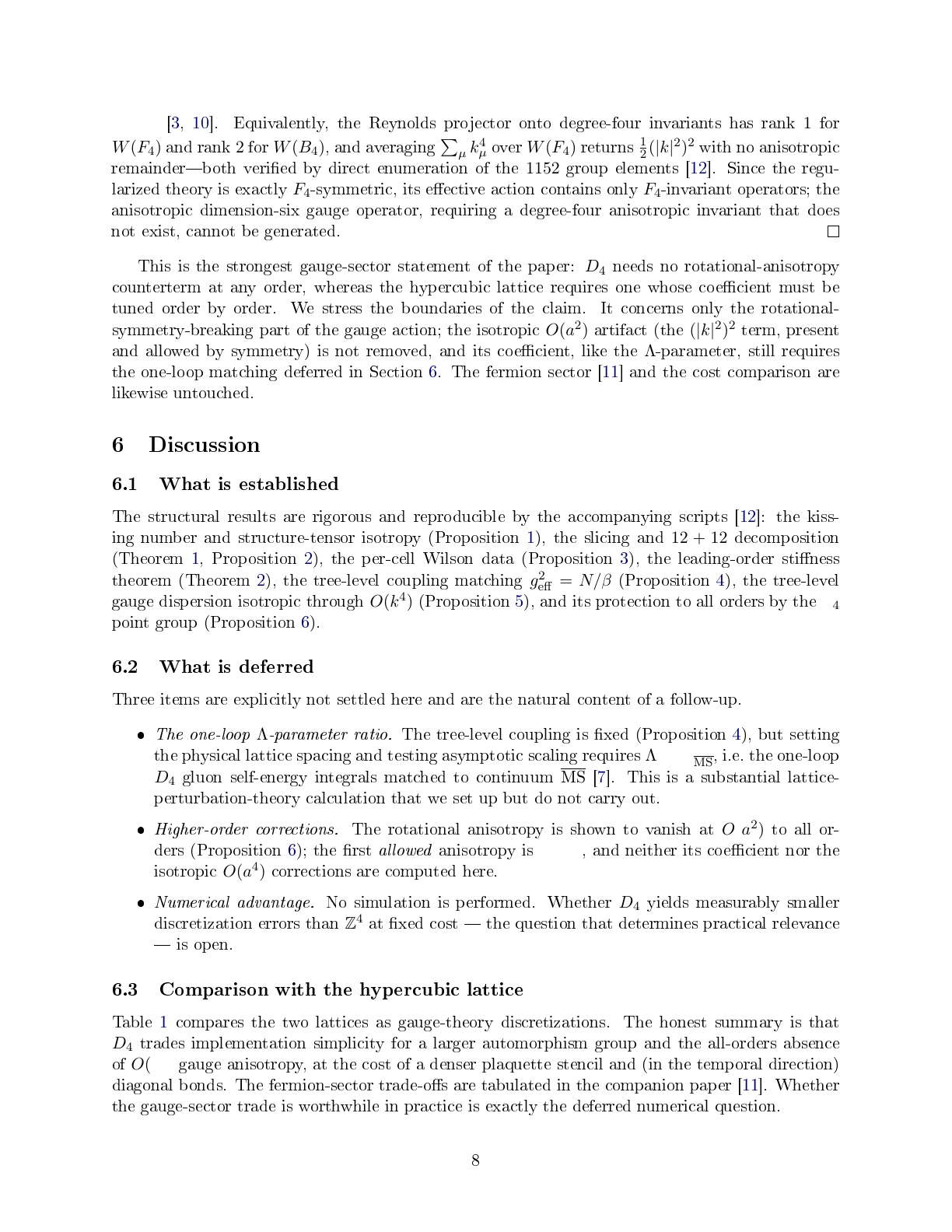
P
µ
k
4
µ
[3, 10]. Equivalently, the Reynolds projector onto degree-four invariants has rank
1
for
W (F
4
)
and rank
2
for
W (B
4
)
, and averaging
P
µ
k
4
µ
over
W (F
4
)
returns
1
2
(|k|
2
)
2
with no anisotropic
remainderboth veried by direct enumeration of the
1152
group elements [12]. Since the regu-
larized theory is exactly
F
4
-symmetric, its eective action contains only
F
4
-invariant operators; the
anisotropic dimension-six gauge operator, requiring a degree-four anisotropic invariant that does
not exist, cannot be generated.
This is the strongest gauge-sector statement of the paper:
D
4
needs no rotational-anisotropy
counterterm at any order, whereas the hypercubic lattice requires one whose coecient must be
tuned order by order. We stress the boundaries of the claim. It concerns only the rotational-
symmetry-breaking part of the gauge action; the isotropic
O(a
2
)
artifact (the
(|k|
2
)
2
term, present
and allowed by symmetry) is not removed, and its coecient, like the
Λ
-parameter, still requires
the one-loop matching deferred in Section 6. The fermion sector [11] and the cost comparison are
likewise untouched.
6 Discussion
6.1 What is established
The structural results are rigorous and reproducible by the accompanying scripts [12]: the kiss-
ing number and structure-tensor isotropy (Proposition 1), the slicing and
12 + 12
decomposition
(Theorem 1, Proposition 2), the per-cell Wilson data (Proposition 3), the leading-order stiness
theorem (Theorem 2), the tree-level coupling matching
g
2
eff
= N/β
(Proposition 4), the tree-level
gauge dispersion isotropic through
O(k
4
)
(Proposition 5), and its protection to all orders by the
F
4
point group (Proposition 6).
6.2 What is deferred
Three items are explicitly not settled here and are the natural content of a follow-up.
The one-loop
Λ
-parameter ratio.
The tree-level coupling is xed (Proposition 4), but setting
the physical lattice spacing and testing asymptotic scaling requires
Λ
lat
/Λ
MS
, i.e. the one-loop
D
4
gluon self-energy integrals matched to continuum
MS
[7]. This is a substantial lattice-
perturbation-theory calculation that we set up but do not carry out.
Higher-order corrections.
The rotational anisotropy is shown to vanish at
O(a
2
)
to all or-
ders (Proposition 6); the rst
allowed
anisotropy is
O(a
4
)
, and neither its coecient nor the
isotropic
O(a
4
)
corrections are computed here.
Numerical advantage.
No simulation is performed. Whether
D
4
yields measurably smaller
discretization errors than
Z
4
at xed cost the question that determines practical relevance
is open.
6.3 Comparison with the hypercubic lattice
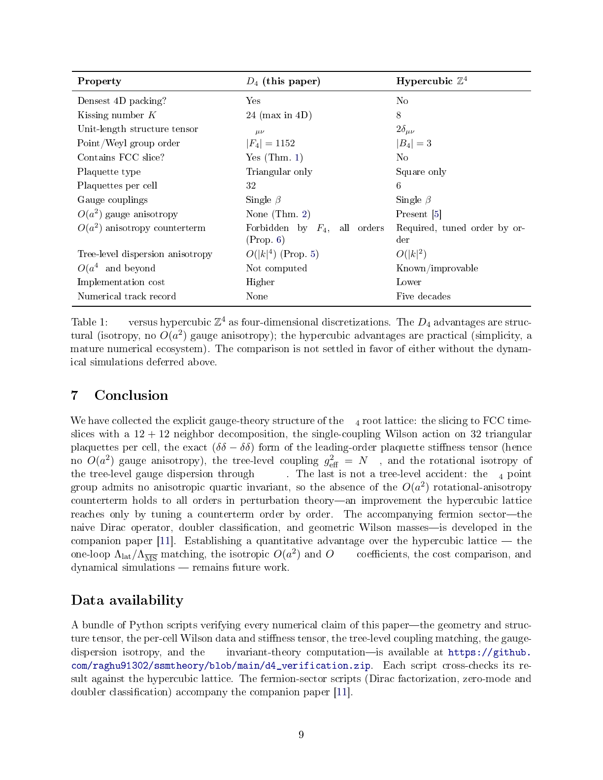
Table 1 compares the two lattices as gauge-theory discretizations. The honest summary is that
D
4
trades implementation simplicity for a larger automorphism group and the all-orders absence
of
O(a
2
)
gauge anisotropy, at the cost of a denser plaquette stencil and (in the temporal direction)
diagonal bonds. The fermion-sector trade-os are tabulated in the companion paper [11]. Whether
the gauge-sector trade is worthwhile in practice is exactly the deferred numerical question.
8
Property
D
4
(this paper) Hypercubic
Z
4
Densest 4D packing? Yes No
Kissing number
K 24
(max in 4D)
8
Unit-length structure tensor
6δ
µν
2δ
µν
Point/Weyl group order
|F
4
| = 1152 |B
4
| = 384
Contains FCC slice? Yes (Thm. 1) No
Plaquette type Triangular only Square only
Plaquettes per cell
32 6
Gauge couplings Single
β
Single
β
O(a
2
)
gauge anisotropy None (Thm. 2) Present [5]
O(a
2
)
anisotropy counterterm Forbidden by
F
4
, all orders
(Prop. 6)
Required, tuned order by or-
der
Tree-level dispersion anisotropy
O(|k|
4
)
(Prop. 5)
O(|k|
2
)
O(a
4
)
and beyond Not computed Known/improvable
Implementation cost Higher Lower
Numerical track record None Five decades
Table 1:
D
4
versus hypercubic
Z
4
as four-dimensional discretizations. The
D
4
advantages are struc-
tural (isotropy, no
O(a
2
)
gauge anisotropy); the hypercubic advantages are practical (simplicity, a
mature numerical ecosystem). The comparison is not settled in favor of either without the dynam-
ical simulations deferred above.
7 Conclusion
We have collected the explicit gauge-theory structure of the
D
4
root lattice: the slicing to FCC time-
slices with a
12 + 12
neighbor decomposition, the single-coupling Wilson action on
32
triangular
plaquettes per cell, the exact
(δδ − δδ)
form of the leading-order plaquette stiness tensor (hence
no
O(a
2
)
gauge anisotropy), the tree-level coupling
g
2
eff
= N/β
, and the rotational isotropy of
the tree-level gauge dispersion through
O(k
4
)
. The last is not a tree-level accident: the
F
4
point
group admits no anisotropic quartic invariant, so the absence of the
O(a
2
)
rotational-anisotropy
counterterm holds to all orders in perturbation theoryan improvement the hypercubic lattice
reaches only by tuning a counterterm order by order. The accompanying fermion sectorthe
naive Dirac operator, doubler classication, and geometric Wilson massesis developed in the
companion paper [11]. Establishing a quantitative advantage over the hypercubic lattice the
one-loop
Λ
lat
/Λ
MS
matching, the isotropic
O(a
2
)
and
O(a
4
)
coecients, the cost comparison, and
dynamical simulations remains future work.
Data availability
A bundle of Python scripts verifying every numerical claim of this paperthe geometry and struc-
ture tensor, the per-cell Wilson data and stiness tensor, the tree-level coupling matching, the gauge-
dispersion isotropy, and the
F
4
invariant-theory computationis available at
https://github.
com/raghu91302/ssmtheory/blob/main/d4_verification.zip
. Each script cross-checks its re-
sult against the hypercubic lattice. The fermion-sector scripts (Dirac factorization, zero-mode and
doubler classication) accompany the companion paper [11].
9
References
[1] T. C. Hales,
A proof of the Kepler conjecture
, Ann. Math.
162
, 1065 (2005),
doi:10.4007/annals.2005.162.1065.
[2] J. H. Conway and N. J. A. Sloane,
Sphere Packings, Lattices and Groups
, 3rd ed., Springer
(1999), doi:10.1007/978-1-4757-6568-7.
[3] H. S. M. Coxeter,
Regular Polytopes
, 3rd ed., Dover (1973).
[4] K. G. Wilson,
Connement of quarks
, Phys. Rev. D
10
, 2445 (1974),
doi:10.1103/PhysRevD.10.2445.
[5] K. Symanzik,
Continuum limit and improved action in lattice theories
, Nucl. Phys. B
226
, 187
(1983), doi:10.1016/0550-3213(83)90468-6.
[6] P. Hasenfratz and F. Niedermayer,
Perfect lattice action for asymptotically free theories
,
Nucl. Phys. B
414
, 785 (1994), doi:10.1016/0550-3213(94)90261-5.
[7] G. P. Lepage and P. B. Mackenzie,
On the viability of lattice perturbation theory
, Phys. Rev. D
48
, 2250 (1993), doi:10.1103/PhysRevD.48.2250.
[8] W. Celmaster,
Gauge theories on the body-centered hypercubic lattice
, Phys. Rev. D
26
, 2955
(1982), doi:10.1103/PhysRevD.26.2955.
[9] G. D. Moore,
Informal lectures on lattice gauge theory
(2003), lecture notes.
[10] J. E. Humphreys,
Introduction to Lie Algebras and Representation Theory
, GTM 9, Springer
(1972), doi:10.1007/978-1-4612-6398-2.
[11] R. Kulkarni,
Geometric Wilson Masses for Doubled Fermions on the FCC and
D
4
Lattices
, in
review at Eur. Phys. J. C (2026), doi:10.5281/zenodo.18410364.
[12] Verication scripts:
https://github.com/raghu91302/ssmtheory/blob/main/d4_
verification.zip
.
10
