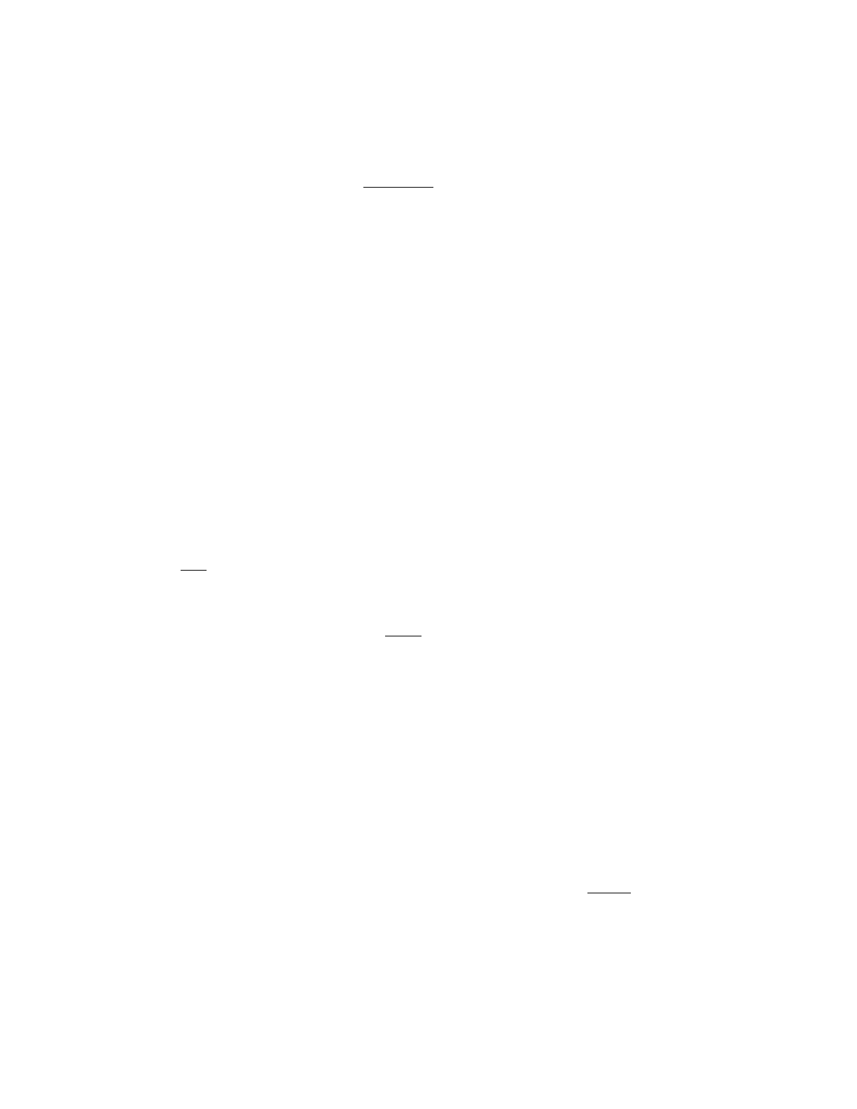
The fine-structure constant from the FCC vacuum code:
α
−1
= π
p
m
p
/m
e
from five axioms
Raghu Kulkarni
SSMTheory Group, IDrive Inc., Calabasas, CA 91302, USA
raghu@idrive.com
Abstract
The Selection–Stitch Model derives particle mass ratios as counts on the FCC vacuum
lattice and fixes no spacing. The measured sizes of its objects place light and leptons on a
Planck-scale lattice and hadrons on a lattice of spacing
L
c
≈
0
.
84 fm; one FCC complex admits
both realizations with identical counts, since counts depend on the boundary maps and lengths
on the Hodge star. The electromagnetic coupling differs between the two scales by the measured
running, so it is not a count. We first ask what the lattice must be to carry a photon at all,
using no measured coupling. Three origins are excluded by mechanism: counts, which cannot
run; the code qubits, since two- and three-level link variables give a strongly coupled photon
(projector Monte Carlo on the photon’s Gauss-law sector:
α
−1
≈
7 and 14–30 against 135), so
the link variable must be a rotor with a small explicit charging energy; and the edge-length field,
which is spin-2. The coupling is carried by a
U
(1) rotor on the node–void half-links, of which the
stabilizer code is taken to be the staggered
Z
2
restriction; the coupling is the field’s impedance,
α
=
p
U/J/
4
π
, with
U
the charging energy of a unit link flux and
J
the stiffness of a plaquette,
here one FCC bond. With
U
the cost of one standing bit,
ϵ
b
=
m
e
c
2
, and
J
the bond quantum
ℏc/(4L), where 4 = K/d is the FCC structure-tensor eigenvalue,
α
−1
= 2π
q
¯
λ
e
/L
c
, L
c
= 4π
2
α
2
¯
λ
e
,
at the confinement scale. With
L
c
=
r
p
this gives
α
−1
= 134
.
65 against the running value
135
.
5
±
0
.
3; with
α
it gives
L
c
= 0
.
83 fm against
r
p
= 0
.
8409 fm. Written in the model’s own
variables the Hamiltonian is a per-bond phase term and a four-bond charging term; its structure
is fixed by the geometry, its two coefficients follow from the postulates once the charging term
is recognized as diagonal in the flux basis and the phase term as purely off-diagonal: the first
is priced by the information postulate as an energy, giving
u
= 1 from the electron calibration
and gauge invariance, the second by the kinematic postulate as a transmission, giving
ȷ
= 1
from the flux current
I
=
−
(
J/ℏ
)
sin B
, whose transfer per tick is exact because the phase is
conserved. The exact Floquet Hamiltonian of the tick shows no significant dressing of their ratio.
No measured coupling enters; the measured
ȷ/u
= 1
.
00
±
0
.
02 is then a test, and the readings the
derivation excludes would have given 95 and 190. The confinement length itself follows from one
count applied twice: two-step paths from the trapped-node defect, 1836 into the bulk at one bit
each and 16 inside it at one quantum each, equated by the model’s stability window. Within the
SSM, then,
α
is not a free parameter: from the axioms alone,
α
−1
=
π
p
m
p
/m
e
= 134
.
6, with
the proton radius an output (0
.
8413 against 0
.
8409 fm), against the running value 135
.
5
±
0
.
3
and
r
p
= 0
.
8409(4) fm. The axioms themselves, the rotor premise and the two-code reading
remain the framework’s assumptions, and the paper marks throughout which claims rest on
them.
1

1 The question
No accepted theory derives the fine-structure constant. Attempts to do so usually aim at
α
−1
=
137
.
036, the value at zero momentum. That is the wrong target for any theory with a cutoff: the
coupling runs, and a mechanism at a scale
µ
produces
α
(
µ
), not
α
(0). At the Planck scale the
Standard Model gives
α
−1
≈
105; at the proton radius it gives
≈
135. A derivation that lands on
137 has placed its cutoff at zero energy.
The Selection–Stitch Model (SSM) is a discrete vacuum: a face-centerd cubic lattice of Bell-pair
bonds carrying a stabilizer code, in which particles are defects and masses are counts. It reproduces
the charged-lepton, pion and nucleon mass ratios with no fitted parameter. It has not said at what
spacing its objects exist, and it has not determined the electromagnetic coupling. This paper closes
both gaps from the model’s axioms. The route is unusual only in its order: the geometry of the
photon sector is settled first, then the two coefficients of its Hamiltonian, then the confinement
length, and the measured coupling is met at the end as a test rather than used as an input.
Section 2 summarizes the model for readers new to it, states its axioms, and ends with the two
gaps. Section 3 closes the first: one FCC complex admits two metric realizations with identical
counts, a Planck-scale code carrying light and leptons and a femtometre code carrying hadrons.
Section 4 gives the geometry of the photon sector. Section 5 runs the measured coupling to the
two lattice scales, to have the comparison values in hand. Section 6 excludes three ways the model
might have produced it, none of the exclusions using a measured coupling. Sections 7–8 identify
the carrier, write the Hamiltonian in the model’s own variables, derive its two coefficients from the
axioms, obtain a closed-form relation among
α
, the electron mass and the confinement length, and
then fix the length itself from the stability window, with the proton radius as an output. Section 9
places it against earlier work. Section 10 is the ledger, and Section 11 concludes.
The status of every claim, derived, calibrated, identified, assumed, testable or not derived, is
collected there rather than marked in the text. Identified means a model quantity assigned to a role
in a standard framework, stated rather than derived.
2 The Selection–Stitch Model in brief
Nothing in this section is new; each paragraph points to the paper that establishes it.
The lattice. The vacuum is a network of Bell-pair bonds of one length
L
. Two operators grow it:
a planar “stitch” that adds a node at the apex of an existing edge, and a rare out-of-plane “lift” that
adds a node above a triangle. Stitch alone gives hexagonal sheets (
K
= 6). Lift produces a frustrated
tetrahedral foam (
K
= 4) that cannot tile space; the Regge deficit 2
π −
5
arccos
(1
/
3)
≃
0
.
128 rad
drives the foam onward. The sheets interlock in ABC stacking and the network saturates at
K
= 12,
the kissing number of three dimensions. The result is the face-centerd cubic lattice, which attains
the Kepler bound. Simulation confirms the saturation, with the under-coordinated fraction falling as
6
.
8
N
−1/3
[
3
]. Every interior node sits in a cuboctahedral shell of twelve neighbors: eight triangular
faces and six square faces [6].
The code. Put one qubit on each of the 3
N
3
nearest-neighbor bonds of a periodic FCC lattice of
box side
N
. Apply a
Z
-check to the twelve bonds at each node and an
X
-check to the twelve bonds
bounding each octahedral void. The checks commute. Each family has one global dependency, so
the code has
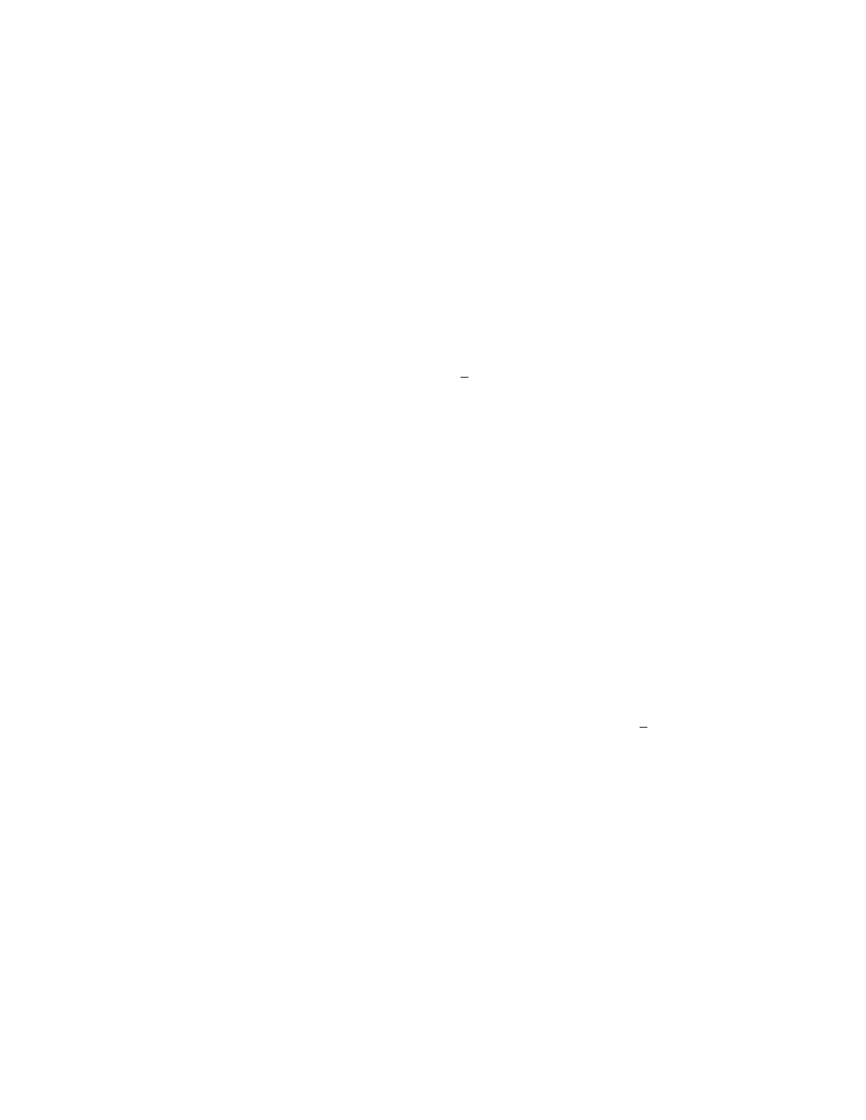
k
= 2
N
3
+ 2 logical qubits: [[192
,
130
,
3]] at
N
= 4. The distance is 3, proven by
2
exhaustive search at
N
= 4 and
N
= 6 [
1
]. In the model the lattice is at once the ground state and
the error-correcting code [2].
Mass as verification cost. A particle is a defect the code cannot repair. Its mass is the number
of stabilizer bits the code must carry to keep it:
C
=
E
s
× C
s
, the bonds in the defect’s footprint
times the checks that can see them. Four axioms from error correction and lattice gauge theory
sieve twenty-five candidate defect geometries down to five. Their counts are 1, 207, 273, 1836, 1839.
The measured mass ratios of the electron, muon, pion, proton and neutron match these to within
0
.
12%, with no fitted parameter [
2
]. The energy per bit,
ϵ
b
, cancels in every ratio. Its value is set
by the electron: ϵ
b
= m
e
c
2
[4].
Matter as a trapped node. The FCC cell has eight tetrahedral voids. A node left over from
the
K
= 4 phase can sit in one, bonded to its four corners; that node is a baryon. Its geometry
yields the fractional quark charges, the three colors from the tetrahedron’s three skew-edge pairs,
and linear confinement from the metric wall at
L/
√
3
[
3
]. Two features of it are used below: the
defect’s graph, four bounding vertices with six edges between them and four spokes to the trapped
node; and the structural count (
K
+ 1)
K
2
− c
skew
K
= 13
×
144
−
36 = 1836, the proton-to-electron
mass ratio, whose thirteen structural nodes are the twelve corner ends of the six edges plus the
trapped center.
Gravity. The FCC lattice is the constant-time slice of the
D
4
root lattice, whose twelve edge-
direction dyads span the symmetric rank-2 tensors; the graviton is the incompatible sector of
the edge-length field, and its linearized kinetic operator is the Einstein operator with Fierz–Pauli
coefficients. Integrating out lattice modes induces a Newton constant proportional to the squared
spacing; matching to
G
N
puts the spacing at the Planck scale, and a bond-level Ryu–Takayanagi
calibration pins
L
0
= 1
.
843
ℓ
P
[
5
]. Two consequences are used below: that spacing, and that the
edge-length field carries spin 2.
The quantum–classical boundary. The structure tensor of the twelve bond directions is
S
µν
= 4
δ
µν
, with 4 =
K/d
. The light speed is four bond lengths per lattice timestep,
c
= 4
L/τ
;
each node transmits one quantum per timestep, so the quantum a bond carries per update is
ℏ/τ
=
ℏc/
(4
L
). A mass excitation stays coherent while its Compton wavelength is resolvable by the
lattice, which gives a two-step threshold at 13.1 and 22.6 µg with exact ratio
√
3 [6].
The photon. Among the sublattices of FCC, the nearest-neighbor
⟨
110
⟩
bonds are non-bipartite
and carry one polarization. The
⟨
111
⟩
links to tetrahedral voids are bipartite but not centrosymmetric.
The
⟨
100
⟩
links to octahedral voids are bipartite, centrosymmetric, and carry Maxwell’s two
polarizations. Light propagates there [7]. Section 4 gives the geometry this paper uses.
2.1 The axioms
The postulates the rest of the paper uses are collected here, so that a reader can see at the outset
what the derivation rests on. (P1)–(P3) are the earlier papers’, restated; (P4) and (P5) are this
paper’s and are argued where they are introduced.
(P1)
Geometry. The vacuum is the FCC lattice with
K
= 12, its bonds carrying the [[3
N
3
,
2
N
3
+2
,
3]]
CSS code of Ref. [1]; K/d = 4 is its structure-tensor eigenvalue [6].
3

(P2)
Kinematics. Each node transmits one quantum per lattice timestep
τ
= 4
L/c
, so a bond
carries E
bond
= ℏ/τ = ℏc/(4L) per update [6].
(P3)
Information. Standing syndrome information the code cannot export is localized energy at
the fixed rate ϵ
b
per bit, calibrated by the electron, ϵ
b
= m
e
c
2
[2, 4].
(P4)
Pricing. What is standing is priced by (P3); what the code resolves within an update is
transient and priced by (P2). This extends (P3) to what (P3) alone does not price. Section 8.8
shows the dichotomy is not arbitrary: in the flux basis the two terms of the Hamiltonian are
respectively diagonal and purely off-diagonal, and (P3) and (P2) are respectively statements
about energy and about transmission. It appears in the ledger as (A0).
(P5)
Two realizations. One FCC complex carries two metric realizations with identical counts, a
Planck-scale fine code and a femtometre confinement code. This is not a postulate of the
earlier papers; Section 3 argues it from four measured sizes and adopts it as the minimal
reading.
What follows from (P1)–(P5), with no measured coupling anywhere in the chain: the structure
of the photon sector’s Hamiltonian (Sections 4, 8.7); both of its stiffnesses, scale and coefficient
(Section 8.8); the exclusion of three candidate carriers (Section 6); the counts that enter the defect’s
two costs, and with them the confinement length (Section 8.11); and therefore
α
itself. What the
paper does not derive is the postulates, the rotor premise of Section 7 under which the photon
sector is a
U
(1) rotor at all, and the two-code reading. The ledger of Section 10 marks every claim
accordingly, and the measured coupling appears there only in calibrated and testable rows.
Two gaps. The counts are ratios and need no spacing, but the objects they describe have sizes,
and the series has not said at what spacing each exists. And the series has not determined the
electromagnetic coupling. Those are the two subjects of this paper.
3 One complex, two spacings
3.1 Four sizes that no single lattice can satisfy
By (P3) a defect of count
C
=
E
s
× C
s
has mass
m
=
C ϵ
b
/c
2
[
4
]. Ratios cancel
ϵ
b
. No spacing
enters. The objects are still extended, and four measurements bound them.
Light. Photons of 1
.
4 PeV are observed [
16
]. A lattice carries no mode shorter than twice its
spacing, so the lattice carrying light has
L ≲
10
−6
fm. Gamma-ray-burst timing puts any linear
dispersion scale above the Planck energy [17].
Leptons. Contact-interaction and (
g −
2) limits bound electron substructure below 10
−4
fm [
18
].
The electron is one bond of size L.
Hadrons. The proton is a trapped node with its four bounding vertices, a structure of radius
L
[
3
], whose verification footprint is the thirty-six-bond coordination cluster [
2
]. Its charge radius is
0.8409(4) fm from muonic hydrogen [14] (CODATA 2022: 0.84075(64) fm [15]).
Tension. The metric wall of Ref. [
3
] gives a linear potential of tension
σ
=
ε
wall
/L
. At
L ≃
0
.
84 fm
and
ε
wall
≃
0
.
8 GeV this is the physical value
σ ≃
(0
.
44
GeV
)
2
[
19
]. At the Planck spacing the
same formula with any bond energy the fine code has, from the GUT scale up, gives a Planckian
tension; matching the physical value would need a bond energy of 3
×
10
−20
GeV, below every scale
the lattice possesses.
4

The first two constraints and the last two cannot share a spacing. The one spacing the series
fixes is gravitational,
L
f
= 1
.
843
ℓ
P
(Section 2; 1
.
665
ℓ
P
in the plaquette-level calibration of Ref. [
6
]).
It satisfies the light and lepton bounds and fails the hadron and tension constraints.
3.2 Counts live in the boundary maps, lengths in the Hodge star
The FCC lattice with its cells is a chain complex. The count
E
s
× C
s
uses only the boundary maps
∂
p
: which checks overlap which edges. It is the same on every realization of the complex. Lengths,
areas and tensions enter through the Hodge star, which assigns measures to cells and scales with
L
:
mass count ←→ ∂, lengths and tensions ←→ ⋆(L). (1)
One combinatorial object can have two metric realizations. The counts are identical on both. This
is why the mass sector never needed a spacing and the strong sector always did.
3.3 The fine code and the confinement code
We take the minimal reading, adopted as (P5): two FCC codes, same combinatorics, two spacings.
The fine code,
L
f
= 1
.
843
ℓ
P
, carries spacetime and gravity, the photon and the leptons; the
confinement code,
L
c
≃ r
p
= 0
.
84 fm, carries the hadrons as trapped nodes, color, the metric wall
and string breaking.
Three consequences are used later.
One field on both codes. The proton’s charge equals the electron’s to
|q
p
+
q
e
|/e <
10
−21
[
18
].
The proton’s charge is a sum of three bond projections on the confinement code [
3
]. The electron’s is
one unit on one fine-code bond. Two independent
U
(1) fields could not agree to that precision. One
field can, because the projection geometry is the same on both lattices. Section 3.1 puts the photon
on the fine code. So the gauge fields propagate in the fine code’s spacetime, and the confinement
code is a crystallized structure embedded in it, as a crystal sits in space. Above the confinement
scale the gauge fields carry no code structure. The code structure that assigns charges to defects
and stiffnesses to bonds exists where the code is.
One energy per bit. The ratio
m
p
/m
e
= 1836 relates a confinement-code count to a fine-code
count. For it to be a pure number,
ϵ
b
must be one constant on both codes. Equivalence-principle
tests require the same: the fine code’s induced metric must respond to a bit on either code with one
weight.
The stability window. A lattice whose energies all scale as
ℏc/L
is stable at every spacing or at
none. A window needs one scale that does not move with
L
. The model has exactly one,
ϵ
b
. The
window is centerd where the counted rest energy of the minimal trapped node equals the energy
to pull a bond to the wall, 1836
ϵ
b
≃ σL
. That gives
L
c
≃ m
p
/σ ≃
0
.
96 fm against
r
p
= 0
.
84 fm.
The chiral condensate gives a third estimate,
ℏc/⟨¯qq⟩
1/3
≃
0
.
79 fm for
⟨¯qq⟩
1/3
≃
250 MeV. We
take
L
c
∈
[0
.
80
,
0
.
96] fm as the model’s band and
r
p
as its best value. The window, in this
mechanical form, locates hadrons once a confinement scale exists; it does not derive
σ
, nor the ratio
L
c
/L
f
≃
3
×
10
19
. Section 8.11 gives it a kinematic form, priced by (P2) and (P4), that fixes
L
c
without σ.
3.4 Three energies of one bond
Three energy scales attach to a bond. They are different objects.
E
bond
=
ℏc/
(4
L
) is kinematic. It is (P2):
ℏ
over the lattice timestep
τ
= 4
L/c
, with the 4
the structure-tensor eigenvalue
K/d
= 12
/
3 of (P1). It is 59 MeV on the confinement code and
∼ 10
18
GeV on the fine code.
5
ε
wall
is mechanical. It is the energy to stretch a bond to the exclusion radius,
≃
0
.
8 GeV on the
confinement code. It sets the tension.
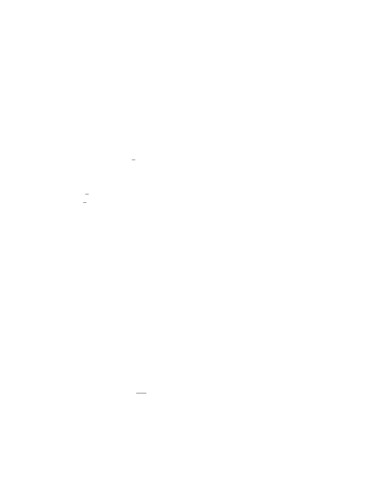
ϵ
b
=
m
e
c
2
= 0
.
511 MeV is informational. It is (P3), the energy the code assigns to one standing
syndrome bit [4]. It is a property of verification, not of any lattice excitation.
An ordinary crystal has the first two (Debye and cohesive energies) and no third. The code adds
the third. The ratio
ϵ
b
/E
bond
is 10
−2
on the confinement code and 10
−22
on the fine code. That
is the electron–Planck hierarchy in the model’s own terms. None of these ratios is derived in this
section; Section 8.11 fixes
ϵ
b
/E
bond
on the confinement code from the stability window. Section 8
uses two of the three scales, E
bond
and ϵ
b
, and not ε
wall
.
4 The node–void sector that carries a photon
We summarize the geometry of Ref. [
7
]. Take units in which the conventional cubic cell has side 2,
so the bond length is
L
=
√
2
. The FCC nodes are the even-parity points of
Z
3
. The octahedral
voids are the odd-parity points. The
⟨
110
⟩
bonds carry the qubits of the [[3
N
3
,
2
N
3
+ 2
,
3]] CSS
code on a periodic box of side
N
[
1
]:
Z
-checks on the twelve bonds at each node,
X
-checks on the
twelve bonds of each octahedral void. The
⟨
100
⟩
links join each node to its six neighboring voids, at
distance
L/
√
2
. They carry no code qubits. Nodes and voids together form a simple cubic lattice of
spacing
L/
√
2
. It is bipartite and centrosymmetric, and its one-form count is Maxwell’s: three links
per site split into one exact and two coexact modes per site, plus three harmonic modes in all, the
first Betti number of the torus.
Every
⟨
110
⟩
bond is the sum of two
⟨
100
⟩
links in exactly two ways, through either of two voids.
The difference of the two paths is a cubic plaquette. There is one plaquette per bond. One link is
used by exactly four bonds, which we call the link’s served quartet. One bond is seen by exactly
four checks, two
Z
and two
X
. These counts are exact on the periodic lattice at every even
N
,
verified by enumeration at N = 4 and N = 6 (Appendix E).
The bonds are also the links of a third cubic lattice, the simple cubic lattice of tetrahedral voids,
which is the Poincar´e dual of the node–void lattice: its links pierce the plaquettes, one per bond; its
plaquettes are the served quartets, one per
⟨
100
⟩
link; its cubes are centerd on the nodes and voids,
and the code’s
Z
- and
X
-checks are the twelve edges of the node- and void-centerd cubes. Its sites
are the tetrahedral voids, where Ref. [
3
] puts the trapped node of Section 8.11. The code is thus a
cube-edge code on the dual of the photon lattice (Appendix E). This lattice joins tetrahedral voids
to each other; it is not the
⟨
111
⟩
diamond of Section 2, which joins them to nodes and is excluded.
Section 6.2 uses this dual description.
5 The measured coupling at the two lattice scales
The derivation of Sections 6–8 uses no measured coupling; this section prepares the values it will
be compared with at the end. The zero-momentum
α
−1
= 137
.
036 is not one of them: a lattice
mechanism at a scale µ produces α(µ), so we run the measured coupling to the two lattice scales.
At the fine code, two-loop
MS
running with Standard Model content (gauge couplings and top
Yukawa, inputs at
m
t
from Ref. [
11
], which reproduce
α
−1
(
M
Z
) = 127
.
95) gives at
µ
=
ℏc/L
f
=
6.6 × 10
18
GeV
α
−1
(ℏc/L
f
) = 104.9 ± 0.3. (2)
The two-loop correction is
−
0
.
7. Higher orders and thresholds are estimated at
±
0
.
2. Input
uncertainties contribute under 0
.
3. The two calibrations of
L
f
of Section 3 differ by 0
.
06. The
6
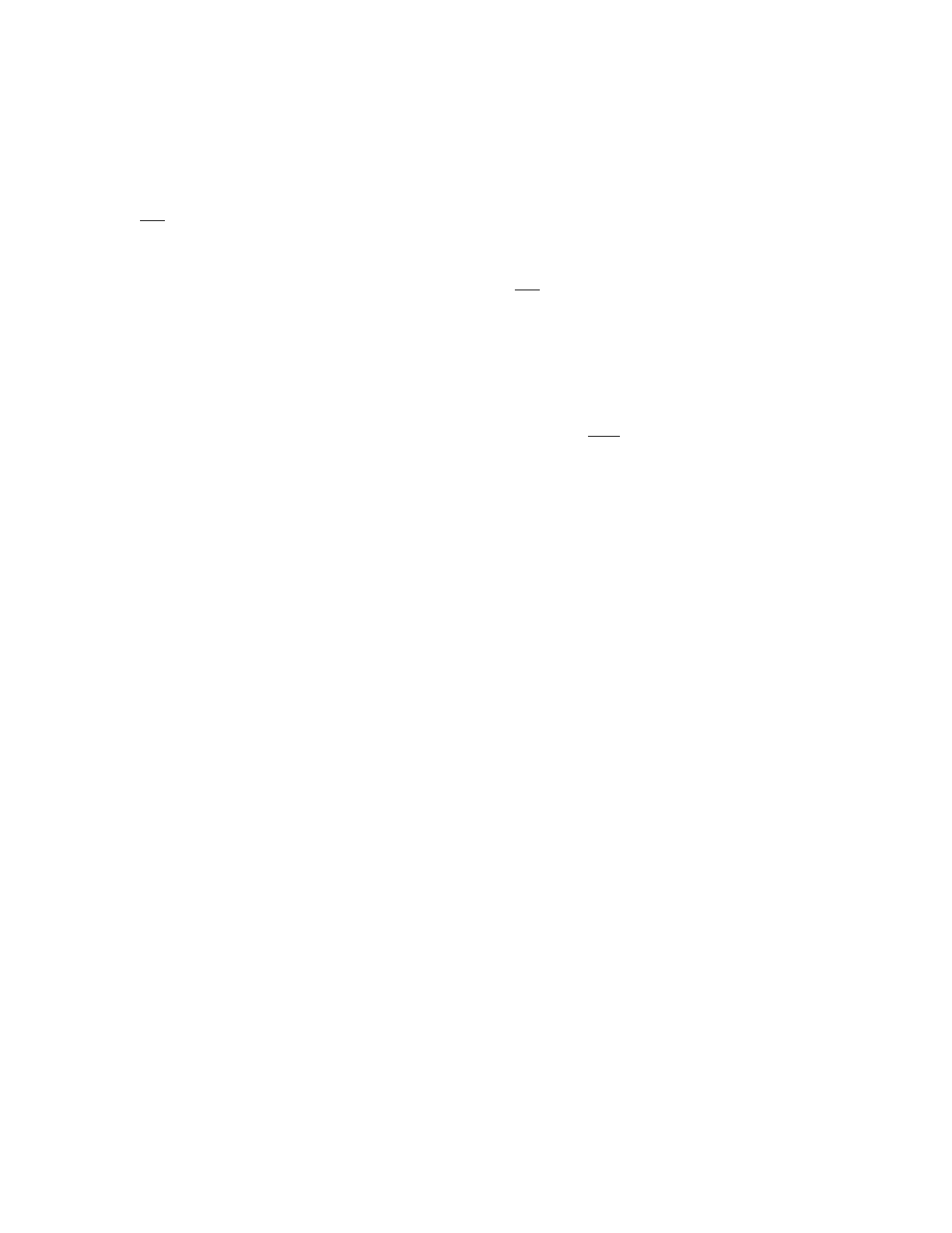
sharpness is a claim of the model: it assumes no charged matter between
M
Z
and the cutoff, which
is what the defect sieve of Ref. [2] asserts. New charged states would lower it.
At the confinement code,
µ
=
ℏc/L
c
≃
0
.
235 GeV for
L
c
=
r
p
. This is the hadronic region. The
leptonic vacuum polarization is computed; the hadronic part is a dispersion integral over
e
+
e
−
data [
13
]. Exact one-loop leptonic polarization at spacelike
Q
2
= 0
.
055 GeV
2
gives ∆
α
lep
= 0
.
0096;
the
MS
logarithms with
e
and
µ
active give 0
.
0107. The hadronic term at this
Q
2
is ∆
α
had
≈
0
.
0005–
0.0010. So
α
−1
(ℏc/L
c
) ≃ 135.5 ± 0.3, β ≡ α
−1
/4π ≃ 10.8, (3)
where the spread covers the scheme (spacelike versus
MS
) and the hadronic term. A lattice-scale
coupling is scheme-dependent at this level, and the comparison below cannot be sharper than that.
This sits deep in the Coulomb phase of compact
U
(1), where
β
c
≃
1
.
01 [
9
]. The tree-level relation
between lattice stiffnesses and coupling used below is therefore expected to hold up to a small
renormalization; Section 8.6 checks it directly.
Two consequences follow before any mechanism. A derivation landing on 137
.
036 is a 30% miss
on the fine code and a 1% miss on the confinement code; proximity to 137 is not evidence. And in
the Kogut–Susskind form of Section 7, where the coupling is
p
U/J/
4
π
for an electric stiffness
U
and a magnetic stiffness
J
, the required ratio is
U/J
= (4
πα
)
2
≃
0
.
0086 at the confinement scale.
The electric term must be two orders of magnitude weaker than the magnetic term. Proposition 3
shows directly that two- and three-level link variables cannot supply this.
6 Three candidate origins excluded by mechanism
6.1 A count cannot run
Proposition 1. If the coupling is a property of the lattice at each of its realizations, it is not a
function of the boundary maps alone.
By Section 3.2, counts are functions of
∂
and are identical on both codes. The coupling is not.
By Section 5 it is
α
−1
≈
105 at
ℏc/L
f
and
≈
135 at
ℏc/L
c
. The difference is Standard Model
vacuum polarization, measured directly up to the electroweak scale [
12
]. A quantity with two values
on two realizations is not a function of
∂
. The proposition holds on the two-code reading (P5). It
uses only that the coupling runs between the two scales, not the value it takes at either.
The premise matters, and it is not an axiom. Section 8 drops it: assumption (A1) sets the
coupling on the confinement code only and lets the fine-code value follow by running. Under (A1)
the proposition no longer excludes a count on the confinement code by itself. The exclusion then
rests on the result: the relation obtained in Section 8 contains the spacing
L
c
, a Hodge datum by
Section 3.2, and is therefore not a count either. The two arguments close the same door from both
sides. What the proposition does dispose of in advance is every integer combination of the
f
-vector
data (12
,
13
,
36
,
38
,
51
,
130
,
192
, . . .
) as a scale-independent value of
α
. Verification-cost ratios, the
natural count candidates, indeed fail: with the dictionary of Section 4, a unit Gauss-law charge at a
node is a twelve-edge object of cost
E
s
× C
s
= 12
×
19 = 228. A unit of plaquette flux is one edge,
of cost 4 with code checks or 1 in the trivial-sector convention of Ref. [
2
]. Read as a Kogut–Susskind
ratio (Section 7), these put the sector deep in the confining phase,
α ≳
0
.
5. That is the wrong
physics, not the wrong number.
6.2 The code qubits fall short
Each
⟨
100
⟩
link serves four code bonds. The obvious link flux is a sum over those four, a five-
level variable, taken with or without orientation signs. Unsigned, it reproduces the code’s checks
7
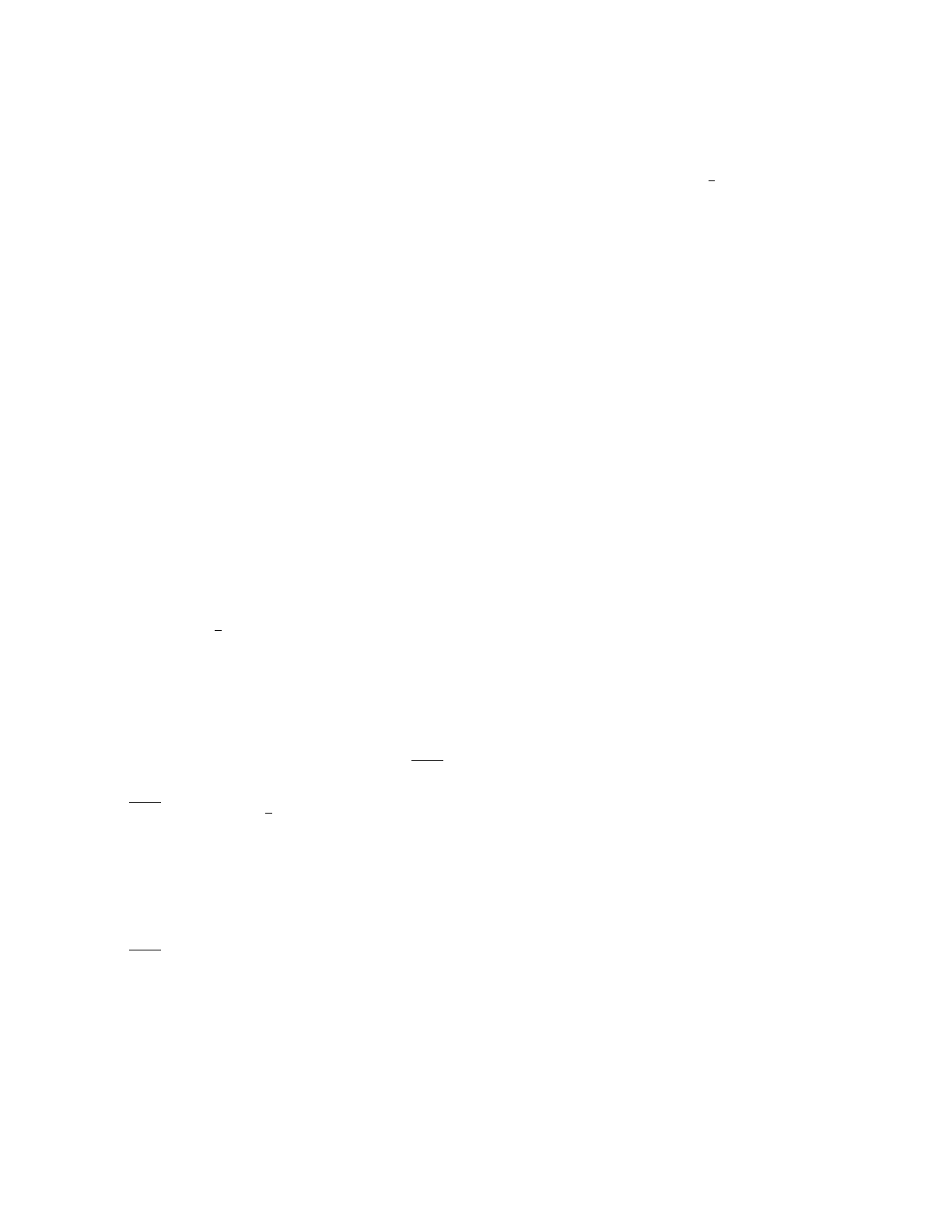
(Proposition 2); signed, it is the photon’s electric field. Neither carries the coupling, and the second
fails for a reason that applies to any low-level link variable (Proposition 3).
Proposition 2. Let
E
link
=
P
4
s
e
over the four served bonds, unsigned,
s
e
=
±
1
2
. The divergence
of
E
at a node is twice the signed sum of the twelve bonds incident on it, and at a void twice the
signed sum of the twelve bonds of the octahedron. The zero-divergence condition is “six up, six down”
on the twelve bonds of every check, and the code’s Z
2
checks are its parity.
Each incident bond uses two links at the node, one per path. The rest is bookkeeping, verified on
the lattice. The proposition says that the code’s checks are the mod-2 reduction of a
U
(1) constraint
the same bonds can carry. It does not say that this constraint is the photon’s Gauss law, and it is
not. In the dual description of Section 4, the photon’s Gauss law is the signed divergence at each
tetrahedral void, six bonds each, and its electric field on a
⟨
100
⟩
link is the signed circulation of the
bond field around the dual plaquette that link pierces, the four served bonds with orientation signs.
The unsigned cube-edge constraint of the proposition, lifted to
U
(1), is a different theory on the
same bonds (Appendix E): it has planar subsystem conservation laws and an anisotropic dispersion
(
ω
2
/k
2
= 2 along [100] with one flat polarization, 0
.
5 and 1
.
5 along [110]), not Maxwell’s. The
signed tetrahedral-divergence lift reproduces
ω
2
/k
2
= 1 for both polarizations in every direction to
five figures. So the code and the photon share the bonds but not the constraint: the code’s checks
are the parity of a U(1) structure that is not the photon.
Proposition 3. Low-level quantum-link variables cannot carry the observed coupling; substantially
more than three flux levels are required, and the link variable must be effectively rotor-like. Projector
Monte Carlo on the photon’s Gauss-law sector gives, for three electric-flux levels per
⟨
100
⟩
link,
α
−1
= 14 at
L
= 6 and 20
±
6 at
L
= 8, consistent with exact diagonalization at
L
= 2 (12
.
5); two
levels (
E
=
±
1
2
) give 7 at
L
= 6 (5
.
1 at
L
= 2). The infinite-volume value is of order 20–30. The
observed value at the confinement scale is 135.5.
The ring-exchange model of Appendix B with the electric flux on each
⟨
100
⟩
link restricted to
{−
1
,
0
,
1
}
is a spin-1 quantum link model on the node–void lattice; the five-level served-qubit sum
is bounded by the two- and three-level cases and the spin-2 case. Its ground state is positive in the
flux basis, so a projector Monte Carlo has no sign problem, and the transverse electric structure
factor at the smallest wavevector gives
p
J/U
=
S
T
/λ
k
directly, with no estimate and no calibration.
Exact diagonalization at
L
= 2, with
U
from the winding sector and
J
from a magnetic twist, gives
p
J/U
= 0
.
41 (spin-
1
2
) and 0
.
99 (spin-1); the Monte Carlo at
L
= 6 and 8 gives the values in the
proposition, with the
L
= 8 uncertainty set by the spread of the three lattice axes rather than the
nominal error. The two methods agree with each other and disagree by a factor of four with the
Gaussian sum-rule estimate of Appendix C, which is therefore retained only as a bound on level
counts. Methods, axis values and the k
2
extrapolation are in Appendix E.
The conclusion is the one emergent-gauge-theory studies reach for spin models generally [
23
,
10
]:
a
U
(1) built from low-level link variables is strongly coupled,
α ∼
0
.
1. Reaching 1
/
135 would need
p
J/U ≃
11 against the 1–2 found at two and three levels. How many levels that corresponds to is
not sharply determined here: the fluctuation bound of Appendix C gives at least seven, and that
bound is unreliable as an estimate, so we state only that the requirement is far above three and
the regime an effectively continuous rotor. So the link variable of the photon sector is a rotor, as
Definition 1 states, and its weak coupling is not a property of its state space but of its energy scales:
an explicit charging energy small against the plaquette stiffness,
U/J ≃
0
.
009. That is what (I1)–(I2)
of Section 8.1 assert and what (P2) and (P3) are shown to supply in Section 8.8, and it gives the
coupling a physical reading within the model: light couples weakly because the standing-information
8
scale, the electron’s mass, is small against the bond quantum. Emergent photons in spin models
have no such small scale and are strongly coupled for that reason.
6.3 Edge lengths are spin-2
Ref. [
5
] obtains the graviton from the incompatible sector of the intrinsic edge-length field. The
twelve edge-direction dyads of
D
4
span the ten symmetric rank-2 tensors, so edge strains determine
a general
h
µν
, and its incompatible part is spin-2. A photon is a vector. No assignment of scalar
lengths to edges contains a vector field; a length has no orientation. A one-form built from a
displacement field is compatible by construction and therefore pure gauge. Projecting the FCC
phonon spectrum onto the
⟨
100
⟩
links confirms this: the one-form is
O
(
k
), its curl is
O
(
k
2
), there
is no Maxwell sector, and the transverse sound speeds along [100]
,
[110]
,
[111] are 0
.
50
,
0
.
35
,
0
.
41
in units of the cubic-cell side times
p
κ/m
, the ordinary Zener anisotropy. The layer that carries
gravity is the wrong representation for light.
7 A rotor whose flat sector carries the code
Ref. [
5
], Section 2.1, states where the
U
(1) lives. Physical particles are
U
(1)-charged defects requiring
complex bond phases. The code’s states are the staggered
Z
2
configurations of those phases. The
carrier is therefore neither the qubit nor the edge length. It is a rotor associated with each bond, of
which the code is taken to be the
{
0
, π}
restriction. The two-path structure of Section 4 says where
the rotor’s fundamental variables sit.
Definition 1 (Photon sector). The fundamental phases
θ
l
∈ U
(1) sit on the
⟨
100
⟩
half-links,
with conjugate integer fluxes
E
l
. A
⟨
110
⟩
bond’s phase is the holonomy of its two-step path. It is
single-valued if and only if the plaquette flux through that bond vanishes. The code’s Bell-pair phases
live in the flat sector of this connection. The stabilizer code is its flat, staggered restriction.
The rotor’s Gauss law in dual form is the signed divergence at the tetrahedral voids (Section 6.2);
the code’s checks are the parity of a different
U
(1) constraint on the same bonds. That the code’s
Bell-pair phases are the flat, staggered restriction of the rotor’s connection is part of the definition,
not derived from it, and it is a statement about the primal phases, not about the dual constraints.
A rotor is continuous, so the exclusion of low-level link variables in Proposition 3 and the level
bound of Appendix C are both satisfied without further input. The coupling is then a matter of
two stiffnesses, not of a state space. In the model’s own variables the plaquette term is a per-bond
term whose coefficient (P2) fixes (Sections 8.7, 8.8); in the auxiliary primal boson realization of
Appendix B it arises as ring exchange with flip amplitude 2
t
2
/V
for hopping
t
and Gauss-law
penalty
V
, from four two-hop paths each through a two-charge intermediate (
J
KS
= 4
t
2
/V
in the
normalization below). Either way the long-wavelength Hamiltonian is
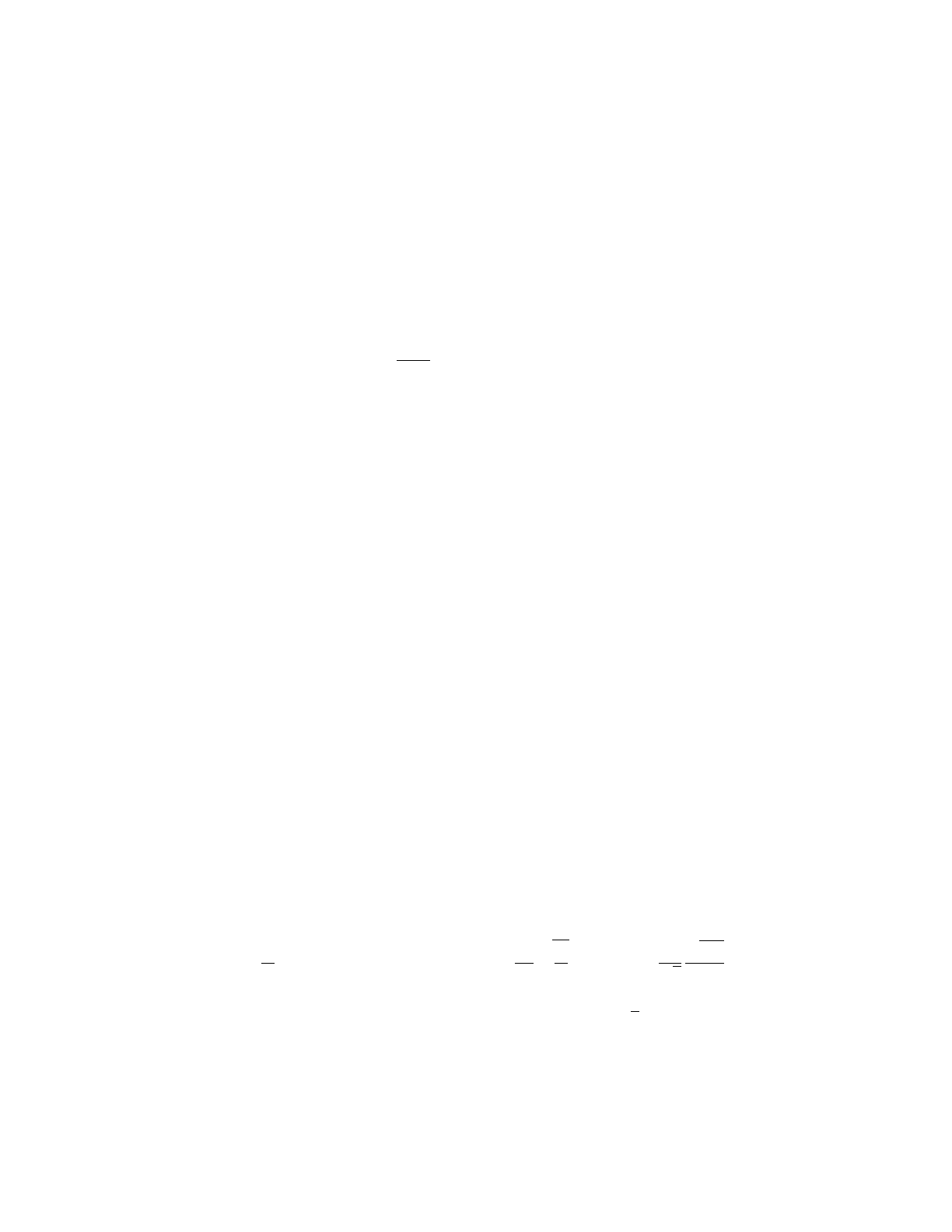
H =
U
2
X
links
E
2
l
− J
X
plaq
cos B
p
, α =
1
4π
r
U
J
, c
lat
=
L
√
2
√
UJ
ℏ
, (4)
in Kogut–Susskind form [
8
], with unit charge equal to unit
E
and
L/
√
2
the node–void spacing. All
of this follows from (P1) and the geometry of Section 4 once the premise of Ref. [
5
], that the bond
phases are the physical
U
(1), is granted. That premise is the paper’s one structural assumption
about the carrier; the two stiffnesses are then derived in Section 8.8.
9

The rotor sets the coupling, not the speed of light. The same Hamiltonian fixes a propagation
speed,
c
lat
= (
L/
√
2
)
√
UJ/ℏ
. With the stiffnesses derived in Section 8.8 on the confinement code,
U
=
ϵ
b
= 0
.
511 MeV and
J
=
E
bond
= 59 MeV,
√
UJ
= 5
.
5 MeV against
ℏc/
(
L/
√
2
) = 332 MeV:
c
lat
≃
0
.
017
c
. A rotor with these stiffnesses is not the propagating photon. That is consistent with
Section 3.3, which puts the light cone on the fine code, but it sharpens what the construction claims.
The confinement code’s rotor sector determines the coupling of the one shared field, through the
ratio
U/J
, while the field’s propagation is the fine code’s. The ratio survives the change of speed;
the product does not. Section 8.3 states this as impedance matching: the ratio is the impedance,
the product is the speed; one field in two media keeps the bare impedance, dresses it by the running
between the scales, and changes the speed. It is labeled (A2) in the ledger; the map itself is not
derived.
8 From two energies to the coupling and the length
8.1
The charging energy is one bit; the plaquette stiffness is one bond quantum
Section 3.4 distinguished the three energies of (P1)–(P3). The photon sector uses two of them.
(I1) U
=
ϵ
b
=
m
e
c
2
. In Eq.
(4)
a unit of flux on one half-link costs
U/
2, so
U
=
ϵ
b
says that a unit
of flux along one bond, the two half-links of a path, costs one bit. The electron is the model’s
one-bond object,
C
e
= 1, and its charge is the unit. The convention matters: had one half-link
cost one bit,
U
= 2
ϵ
b
and
α
−1
= 95. Section 8.8 shows the bond is forced: the half-link reading
would make the electron half a bond, contradicting
C
e
= 1. That the electron’s footprint is a
unit flux along one bond, rather than a point source at a site, is part of the identification.
(I2) J
=
E
bond
=
ℏc/
(4
L
).
J
is the curvature of the plaquette term,
J
(1
− cos B
)
≃ JB
2
/
2. A
plaquette is one FCC bond (Section 4). Flux through it is the two paths disagreeing about
that bond’s phase. By (P2) the stiffness of a bond’s phase is the quantum it carries per lattice
update. Section 8.8 fixes the coefficient from the operator’s form.
The 4 in (I2) is not a convention. In Ref. [
6
], Section 3, it is the eigenvalue of the FCC structure
tensor,
S
µν
=
P
j
n
µ
j
n
ν
j
= 4
δ
µν
, equal to
K/d
= 12
/
3. The light speed is the long-wavelength phase
velocity of the bond mode,
c
= 4
L/τ
. The timestep is
τ
= 4
L/c
. The quantum per update is
ℏ/τ
=
ℏc/
(4
L
). It is the
K
= 12 bond quantum that enters, not the
K
= 6 quantum of the cubic
sublattice’s own star, because a plaquette is a
⟨
110
⟩
bond. This holds given the identification
c
=
v
ph
of Ref. [6].
8.2 The coupling is fixed where the code is
Both codes carry the same
ϵ
b
(Section 3.3), but only one of them carries code structure at the scale
in question: the gauge fields propagate in the fine code’s spacetime without it above the confinement
scale, and it crystallizes at Λ. A coupling fixed by code stiffnesses is therefore fixed where the code
is, and the fine-code value is inherited by running. Applying (I1)–(I2) on the fine code instead
would give α
−1
∼ 10
12
, since E
bond
∼ 10
18
GeV there.
(A1)
The coupling is set at the confinement code, where the code structure that assigns charges
and stiffnesses exists. The fine-code value is its Standard Model running. This is consistent
with Section 3.3 and required if (I1)–(I2) hold at all.
10
8.3 Impedance and speed: what each code fixes
The two combinations of
U
and
J
are the two constants of a medium. In SI units the fine-structure
constant is the vacuum impedance in units of the quantum of resistance,
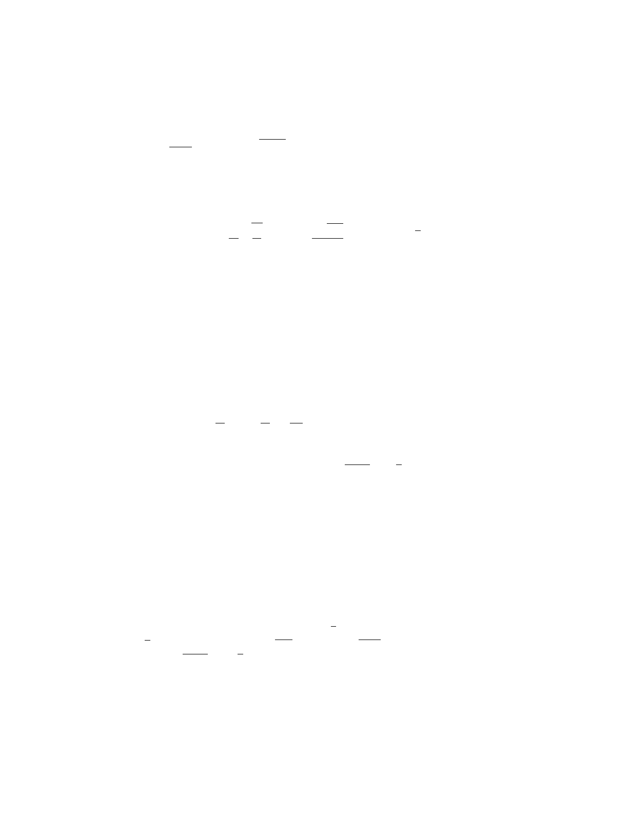
α =
Z
0
2R
K
, Z
0
=
p
µ
0
/ϵ
0
= 376.73 Ω, R
K
= h/e
2
= 25 812.8 Ω, (5)
an identity, not an approximation. On the lattice, with
E
l
the electric flux through a link’s dual
plaquette in charge quanta and
B
p
the flux through a plaquette in flux quanta,
U
plays 1
/ϵ
in the
D formulation and J plays 1/µ (Appendix D), and
Z =
ℏ
e
2
r
U
J
, v =
a
√
UJ
ℏ
, a = L/
√
2. (6)
The spacing enters the speed and cancels in the impedance;
α
=
Ze
2
/
2
h
then returns Eq.
(4)
with
its normalization fixed. The coupling is the impedance; the speed is the geometric mean.
This is what the two-code reading needs, stated as a matching condition. One field on both
codes (Section 3.3) means one bare impedance: two media with different bare
Z
carrying one
U
(1)
would reflect the field at every interface, and a proton and an electron would couple to it with
different strengths at the same scale, which is two fields, not one. But the impedance the field
presents at a scale
µ
is the bare one dressed by the charged matter below
µ
: vacuum polarization
renormalizes the effective electromagnetic coupling between the two scales, and since
Z ∝ α
in
Eq.
(6)
, the effective lattice impedance is dressed in the same ratio. The running of Section 5 is
that dressing. The map from the confinement code to the fine code is therefore
U
J
f
=
U
J
c
α
f
α
c
2
, (UJ)
f
= (UJ)
c
, (7)
where
α
f
/α
c
=
α
−1
c
/α
−1
f
= 135
.
5
/
104
.
9 = 1
.
29 is the Standard Model running between the two
scales, so that (
U/J
)
f
/
(
U/J
)
c
= 1
.
29
2
= 1
.
67, and
p
U
f
J
f
=
√
2 ℏc/L
f
fixed by the fine code’s
speed. This is (A1) in impedance language: the confinement code sets the bare
Z
, the fine code
presents it dressed. Because the two codes share one combinatorics, the identifications of
ϵ
and
µ
carry the same geometric constants on both, and no factor other than
a
and the dressing distinguishes
them (Appendix D). Numerically
U
f
= 0.68 E
bond,f
, J
f
= 47 E
bond,f
, J
f
/U
f
= (4πα
f
)
−2
= 70. (8)
On the fine code both stiffnesses are Planckian and kinematic, as they should be for a sector that
carries no standing information; on the confinement code one of them is the information scale.
The two stiffnesses are determined individually by two inputs, and it is worth being explicit
about which. The impedance ratio, Eq.
(7)
, gives
R ≡ U
f
/J
f
; the fine-code condition
c
lat
=
c
,
with
c
= 4
L
f
/τ
the tick of Ref. [
6
] and
a
=
L
f
/
√
2
the node–void spacing, gives
P ≡ U
f
J
f
=
(
ℏc/a
)
2
= (4
√
2 E
bond,f
)
2
. Then
U
f
=
√
P R
and
J
f
=
p
P/R
, which are the values above; their
product reproduces
p
U
f
J
f
= 4
√
2 E
bond,f
by construction, not as a check. What is not automatic
is that the two requirements are compatible at all: the matching yields a positive pair of Planckian
stiffnesses, both of order the fine code’s own bond quantum, with
U
f
below it and
J
f
a few tens
above, rather than values separated by the eleven orders of magnitude that separate
ϵ
b
from
E
bond
on the confinement code. That is the content of the statement that the fine code carries no standing
information.
11
Given one bare impedance, which code fixes which combination is not a choice. The fine code
has
c
but no
ϵ
b
-scale stiffness for the rotor: it fixes
v
and cannot fix
Z
. The confinement code
has
ϵ
b
and
E
bond
but a rotor speed of 0
.
017
c
: it fixes
Z
and cannot fix
v
. Each fixes the one
combination its ingredients determine, and the shared field takes both. Assumptions (A1) and (A2)
of the ledger are the two halves of this single statement: the field’s impedance is set where the
standing-information stiffness exists, its speed where the light cone exists. What is not derived
is the map itself, a Hamiltonian for the fine code’s rotor with
U
f
and
J
f
as computed; the values
above are what such a Hamiltonian must return, and the dressing factor in Eq.
(7)
is the one place
where the matter content enters the lattice stiffnesses.
8.4 The closed form
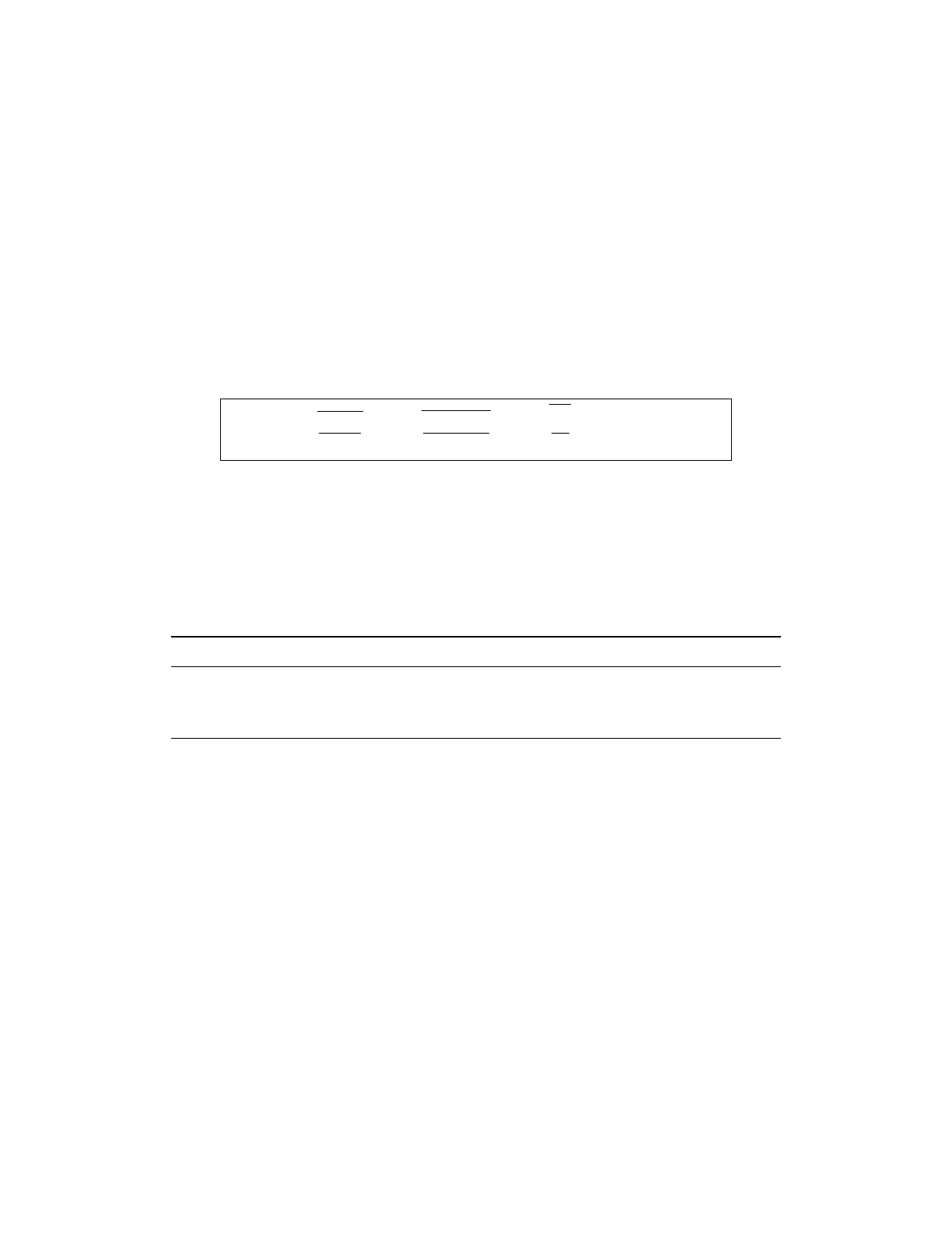
Inserting (I1)–(I2) into Eq. (4) at L = L
c
:
α
−1
= 4π
r
E
bond
ϵ
b
= 4π
r
ℏc
4L
c
m
e
c
2
= 2π
s
¯
λ
e
L
c
, L
c
= 4π
2
α
2
¯
λ
e
(9)
Here
¯
λ
e
=
ℏ/m
e
c
= 386
.
159 fm. The inverse coupling is 2
π
times the square root of the electron’s
Compton wavelength over the confinement spacing. Each factor has a source: 4
π
and the square
root from Kogut–Susskind; m
e
from (I1); ℏc/4L with 4 = K/d from (I2); L
c
from (A1).
8.5 Read in both directions
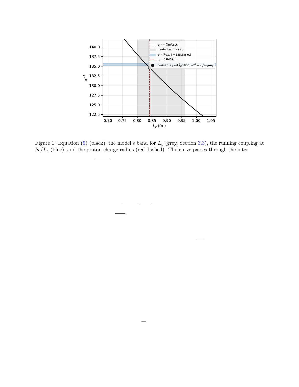
Equation (9) relates three measured quantities (Table 1, Fig. 1).
input implied measured
L
c
= r
p
= 0.8409 fm α
−1
(ℏc/r
p
) = 134.65 135.5 ± 0.3 (Eq. 3)
α
−1
(ℏc/L
c
) = 135.5 ± 0.3 L
c
= 0.827–0.834 fm r
p
= 0.8409(4) fm [14]
α
−1
(0) = 137.036 (for reference) L
c
= 0.812 fm —
Table 1: Equation
(9)
in both directions, for the minimal microscopic normalization
u
=
ȷ
= 1
of Section 8.8. With that normalization the relation agrees to 0
.
6% in
α
−1
, equivalently 1
.
2% in
L
c
, without a continuous fitted parameter; the normalization is derived from (P2) and (P3) in
Section 8.8, not fitted. The last line shows the size of the running: the zero-momentum coupling
would miss by 3.5%.
Two remarks on precision.
α
−1
∝ L
−1/2
c
, so the band
L
c
∈
[0
.
80
,
0
.
96] fm spans
α
−1
∈
[126
,
138].
The relation is satisfied by the proton radius and not by the upper end of the band. This favors
L
c
=
r
p
over the stability-window estimate 0
.
96 fm. It also takes a side in the proton-radius puzzle:
the earlier electronic-hydrogen and scattering value, 0
.
877 fm, gives
α
−1
= 131
.
9, a 2
.
7% miss, four
times the residual with the muonic value. The relation is compatible only with the small radius.
The residual 0
.
6% in
α
−1
is comparable to the scheme spread of Eq.
(3)
and is dominated by it,
by ∆
α
had
at
Q
2
≃
0
.
05 GeV
2
, and by whether
L
c
=
r
p
exactly. The relation is testable: if
L
c
=
r
p
exactly, Eq.
(9)
requires
α
−1
(
µ
= 0
.
235
GeV
) = 134
.
65
±
0
.
05 in the scheme the rotor Hamiltonian
defines; a microscopic derivation that fixes the scheme turns this into a sharp test.
12
0.70 0.75 0.80 0.85 0.90 0.95 1.00 1.05
L
c
(fm)
122.5
125.0
127.5
130.0
132.5
135.0
137.5
140.0
1
1
= 2
e
/
L
c
model band for
L
c
1
(
c
/
L
c
) = 135.5 ± 0.3
r
p
= 0.8409 fm
derived:
L
c
= 4
e
/1836,
1
=
m
p
/
m
e
Figure 1: Equation
(9)
(black), the model’s band for
L
c
(grey, Section 3.3), the running coupling at
ℏc/L
c
(blue), and the proton charge radius (red dashed). The curve passes through the intersection
of the two measured bands. The marked point is the derived value of Section 8.11,
L
c
= 4
¯
λ
e
/
1836 =
0.8413 fm and α
−1
= π
p
m
p
/m
e
= 134.6, which uses neither measured quantity.
8.6 The tree-level relation checked
Equation
(4)
is a tree-level statement, and at
β ≃
11 it is expected to hold up to a renormalization
of order
α
. It can be checked on the lattice of Section 4. A projector Monte Carlo on the photon’s
Gauss-law sector (Appendix F,
alpha liftB gfmc fast.py
), with links of large spin and an explicit
charging energy in the ratio
U/J
= (4
πα
)
2
= 0
.
0086, has no sign problem, and the forward-walked
transverse structure factor gives
p
J/U
directly from its slope at the smallest wavevector. At
L
= 4
it returns
α
−1
= 132 and 136 on two lattice axes against the tree-level 135
.
5, the third axis being a
2
.
5
σ
fluctuation of correlated samples. The relation therefore holds on this lattice at the ten-percent
level. A percent-level determination of the renormalization needs a worldline calculation with pure
estimators: at weak coupling the lowest photon mode,
ω
min
=
λ
min
√
UJ ≃
0
.
19
J
at
L
= 6, sets a
projection time over which forward-walking lineages collapse, and the
L
= 6 runs of the same code
do not converge. The check does not bear on (I1)–(I2), whose ratio was the input; it bears on the
formula that turns that ratio into α.
8.7 The Hamiltonian in the model’s variables, and its tick
Equation
(4)
is written on the primal half-links. The model’s own variables are the bonds. For
divergence-free
E
the link flux is the dual curl of an integer field on the bonds,
E
l
= (
m
1
+
m
2
−
m
3
− m
4
)
l
over the four bonds the link serves, and the gauge-invariant angle attached to a bond is
its plaquette phase
B
b
, conjugate to
m
b
. In these variables the two terms of Eq.
(4)
exchange roles:
H = −J
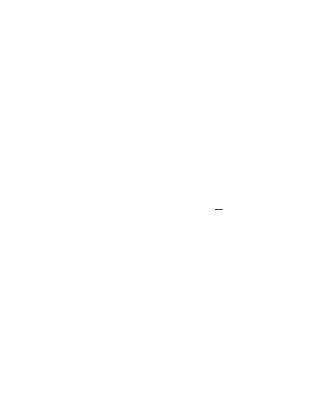
X
bonds
cos B
b
+
U
2
X
links
(m
1
+ m
2
− m
3
− m
4
)
2
. (10)
The stiffness term is now a single-bond term on the bond’s own phase, the physical Bell-pair phase
of Ref. [
5
]; the charging term is the four-bond interaction on each served quartet. Every structural
13
feature of Eq.
(10)
is fixed by the geometry of Section 4. What geometry does not fix is
J
and
U
,
which are properties of the time-evolution rule.
The two coefficients are then fixed by (P2) and (P3), applied to the two kinds of operator
Eq.
(10)
contains; Section 8.8 does that and obtains
J
=
E
bond
and
U
=
ϵ
b
. The plaquette term is
the elementary move here, not a second-order process: the bridge equation, Eq.
(24)
, belongs to the
auxiliary boson model of Appendix B, in which the flip is perturbative.
One thing remains to check, and it can be checked exactly. The tick is a unitary,
U
τ
= exp
i
X
b
cos B
b
exp
−
i
2
ϵ
b
E
bond
X
l
(curl m)
2
l
, (11)
whose first factor is order one per tick while the second is small (
ϵ
b
/E
bond
= 0
.
0087). The two do
not commute, and the effective (Floquet) Hamiltonian
H
F
= (
iℏ/τ
)
log U
τ
could in principle carry
the charging term dressed by an
O
(1) function of the kick. Computing
H
F
exactly and projecting it
onto the two operators of Eq.
(10)
gives
U
eff
/J
eff
equal to the input
ϵ
b
/E
bond
to 10
−4
on a single
bond at one radian per tick, and to 0
.
2–1% on a served quartet (Appendix E). No significant dressing
of the ratio is observed within the tested truncations: the Floquet coupling is the tree-level coupling
to at most about 1%, α
−1
= 4π
p
E
bond
/ϵ
b
= 134.65 at L
c
= r
p
.
With Eq.
(10)
, its coefficients and the absence of dressing, the photon sector is determined by
(P1)–(P4) alone.
8.8 The two coefficients
Each identification contains two separable claims: a choice of energy scale and a choice of an
O
(1)
coefficient. Write
U = u ϵ
b
, J = ȷ E
bond
, α
−1
= 2π
r
ȷ
u
s
¯
λ
e
L
c
, (12)
with u, ȷ pure numbers. Equation (9) is the case u = ȷ = 1.
The scales are forced by (P3) and (P4). Ref. [
4
] states the mass rule in its current form: standing
syndrome information the code cannot export is localized energy at the fixed rate
ϵ
b
per bit. We
take its complement with it: transient reconfigurations, which the code resolves within an update,
are not standing and carry the kinematic scale
ℏ/τ
=
E
bond
. This is (P4), and it appears in the
ledger as (A0).
The electric term is standing.
E
l
is conserved on each link in the absence of hopping. A unit of
flux sitting on a half-link is a syndrome the code holds indefinitely. Its energy is therefore
ϵ
b
per
unit, and U ∝ ϵ
b
, by the postulate of Ref. [4].
The magnetic term is transient. In the model’s own variables it is the per-bond phase term
of Eq.
(10)
, priced by (P2): one quantum per bond per tick,
J
=
ℏ/τ
=
E
bond
(Section 8.7). Its
scale is kinematic because the bond phase is what moves in a tick. The same conclusion follows in
the auxiliary primal boson model of Appendix B, where the plaquette term arises at second order,
J
= 2
t
2
/V
: the hop
t
is one update, the two-charge intermediate is virtual and lasts one update, so
both
t
and
V
are kinematic and
J
= (2
˜
t
2
/
˜
V
)
E
bond
∝ E
bond
. The alternative, a transient charge
charged at
ϵ
b
, would give
J ∼ E
2
bond
/ϵ
b
≃
14 GeV on the confinement code and
α
−1
∼
2000; it is
excluded by the data as well as by the postulate. The two descriptions agree on the scale; the tick
statement is primary, the ring-exchange form is its appearance in a particular realization.
So the assignment of
ϵ
b
to
E
and
E
bond
to
B
follows from (P4). The coefficients follow from
what (P2) and (P3) are statements about.
14
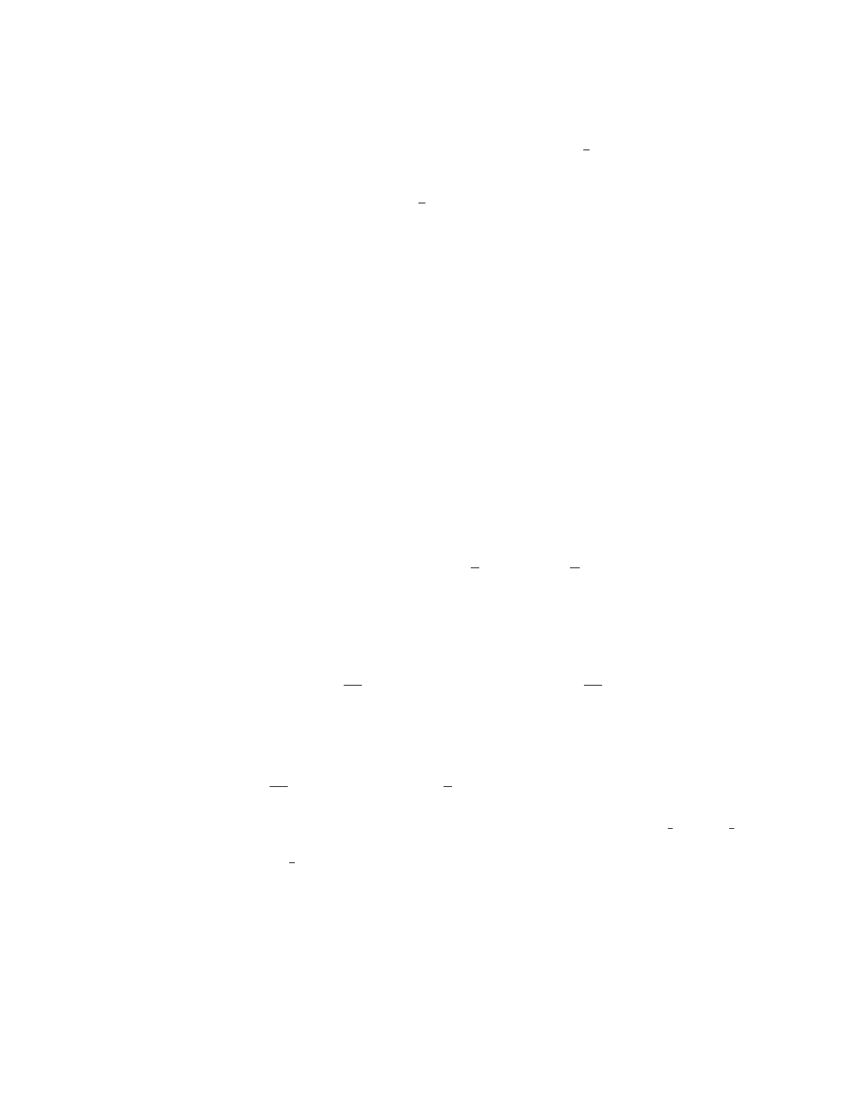
The two terms are different kinds of operator. In the flux basis of Eq.
(10)
, the charging
term is diagonal: (
U/
2)
P
l
E
2
l
has a definite value in any state of definite flux. The phase term
has no diagonal part. Since
B
b
is conjugate to the integer
m
b
,
cos B
b
=
1
2
(
e
iB
b
+
e
−iB
b
) raises and
lowers m
b
, and
⟨m
b
± 1| − J cos B
b
|m
b
⟩ = −
J
2
, ⟨m
b
| − J cos B
b
|m
b
⟩ = 0. (13)
The charging term stores energy; the phase term moves flux. This is the distinction (P4) draws,
now visible in the operators: (P3) is an energy statement and prices the diagonal term, (P2) is a
transmission statement and prices the off-diagonal one.
u
= 1. By (P3),
ϵ
b
is the cost of one standing bit, and it is calibrated by the electron, the minimal
defect of the sieve with
C
e
= 1 [
2
]. The minimal charged excitation of the photon sector is one
bond of flux, and this is geometry rather than convention: a unit of
E
on a single half-link has
div E
= 0 at both of its ends, so it is a charge and an anticharge, one at a node and one at a void;
the shortest gauge-invariant segment carrying a single unit of charge terminating on lattice nodes is
two half-links, which is one bond. There is no smaller charged object. Hence one bond of standing
flux costs exactly one bit,
U
=
ϵ
b
and
u
= 1. The half-link reading,
u
= 2, would make the electron
half a bond and contradict C
e
= 1.
ȷ
= 1. (P2) is a statement about transmission, so it is a statement about a current, and the phase
term has one. With [
B
b
, m
b
] =
i
and
e
±iB
b
|m
b
⟩
=
|m
b
±
1
⟩
, the commutators are [
e
iB
, m
] =
−e
iB
and [e
−iB
, m] = +e
−iB
, so
[H
J
, m
b
] = iJ sin B
b
, I
b
≡ ˙m
b
=
i
ℏ
[H
J
, m
b
] = −
J
ℏ
sin B
b
. (14)
The flux current carried by a bond is
J/ℏ
times
sin B
b
. Because [
H
J
, B
b
] = 0, the phase is a constant
of the motion under this term and the current is too, so the flux transferred in one tick is exact
rather than perturbative:
Z
τ
0
⟨I
b
⟩dt = −
Jτ
ℏ
⟨sin B
b
⟩, max
states
Z
τ
0
⟨I
b
⟩dt
=
Jτ
ℏ
, (15)
the maximum being attained at
B
b
=
±π/
2. (P2) says a bond transmits one quantum per tick; that
is the statement that this maximum is one flux quantum,
Jτ
ℏ
= 1 =⇒ J =
ℏ
τ
= E
bond
, ȷ = 1. (16)
Both identities of Eq.
(14)
and the exactness of Eq.
(15)
are verified numerically in
alpha current operator.py
:
evolving a phase state at
B
=
π/
2 for
τ
= 0
.
5
,
1
,
2 in units
J
=
ℏ
= 1 gives
⟨
∆
m⟩
=
−
0
.
50
, −
0
.
99
, −
1
.
99.
The readings that gave
1
2
and 2 are now excluded quantitatively. Taking the span 2
J
as the
quantum makes the maximum transfer half a flux quantum per tick; taking one channel,
J/
2, makes
it two. Neither is one quantum per tick, and neither uses the measured coupling to fail. What the
derivation does assume is that (P2) is a bound on transfer, saturated by the state that maximizes
the current, in the same sense as a speed limit; the postulate as the series states it is a statement
about what a node transmits in a timestep, which is that.
15
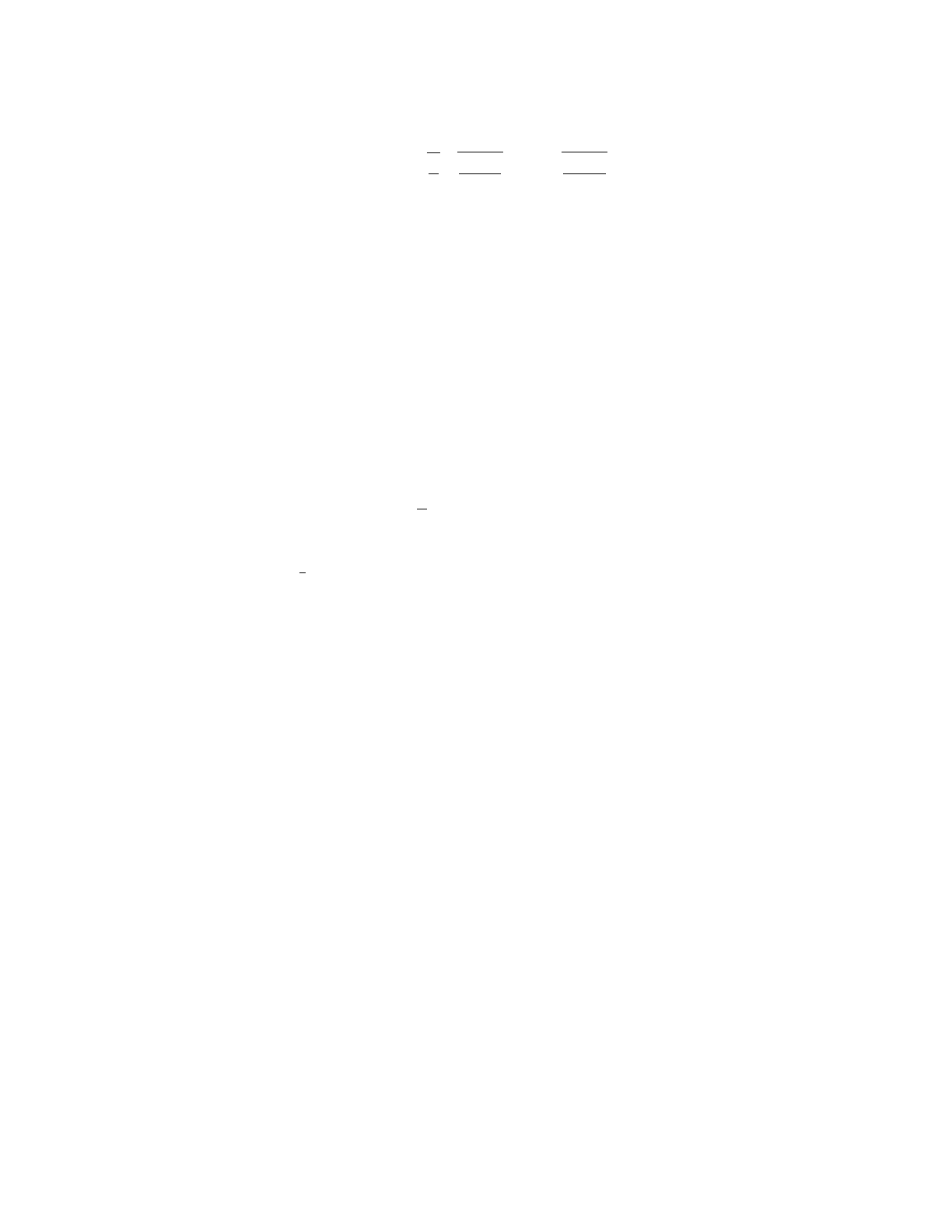
Consequence. With u = ȷ = 1,
α
−1
= 4π
r
ȷ
u
r
E
bond
ϵ
b
= 4π
r
E
bond
ϵ
b
, (17)
and no measured coupling has entered: (P1)–(P4), the rotor premise of Section 7, gauge invariance
and the electron calibration suffice. The measured value of Eq.
(18)
below is then a test rather than
an input, and the alternatives excluded above would have given 95 and 190.
The same statement in the auxiliary boson model of Appendix B is
V
= 4
E
bond
: a transient
unit charge is priced on the four
⟨
110
⟩
bonds the moved link serves, one quantum each, giving
J
KS
= 4
t
2
/V
=
E
bond
for
t
=
E
bond
. The four is the served quartet of Section 4; pricing the charge
per violated site instead (
V
= 2) or per moved link (
V
= 1) gives 190 and 269. The two languages
agree because both apply (P2) to bonds.
8.9 The measured coefficient ratio
Independently of the above, the ratio can be read off the data. Writing
U
=
u ϵ
b
and
J
=
ȷ E
bond
as
in Eq. (12), Eq. (9) with the measured α and L
c
= r
p
gives
ȷ
u
= 1.00 ± 0.02, (18)
the uncertainty being that of Eq.
(3)
and of
L
c
. The derivation above predicts 1; the nearest
alternatives it excludes,
1
2
and 2, are 30% away. This is the paper’s one quantitative test of the
coefficient sector, and it is passed.
8.10 What the relation establishes
Equation
(9)
makes the coupling and the confinement length one quantity: given either, the model
fixes the other through
m
e
and the integer 4. Section 8.11 then fixes the length itself, so that
within the model
α
is determined; what it is determined by are the framework’s postulates, listed in
Section 10. As physics, it says
α
and the proton’s size are one number seen through the electron
mass. The question “why 1
/
137” becomes “why is
r
p
/
¯
λ
e
= 4
π
2
α
2
”. The model answers that to the
extent it answers where the vacuum crystallizes; Section 8.11 shows that its stability window, in
kinematic form, does answer it, at the price of one further identification.
What Eq.
(9)
establishes is a relation among three measured constants with no continuous
fitted parameter, satisfied to 0
.
6% in
α
−1
for the minimal normalization
u
=
ȷ
= 1, with each
factor sourced from a published step of the series, with the scales of its two stiffnesses forced by the
model’s postulate, and and with its one pure number derived from (P2) and (P3) rather than fitted
(Section 8.8). The postulates themselves are the series’, not results of this paper.
8.11 The window in kinematic form: the proton radius as an output
The model’s own stability window closes the loop, once its mechanical side is replaced by a kinematic
one. Section 3.3 located the confinement code where the counted rest energy of the trapped node
equals its mechanical energy, and wrote the mechanical side as
σL
c
, good to a factor of order one.
Axioms (P2) and (P4) give that side a sharper form, and it is worth deriving it before comparing
with anything measured.
Two costs attach to the trapped-node defect of Ref. [
3
], and they are two applications of one
count. The count is of ordered two-step paths from the defect’s nodes:
K
2
= 144 is not the second
16
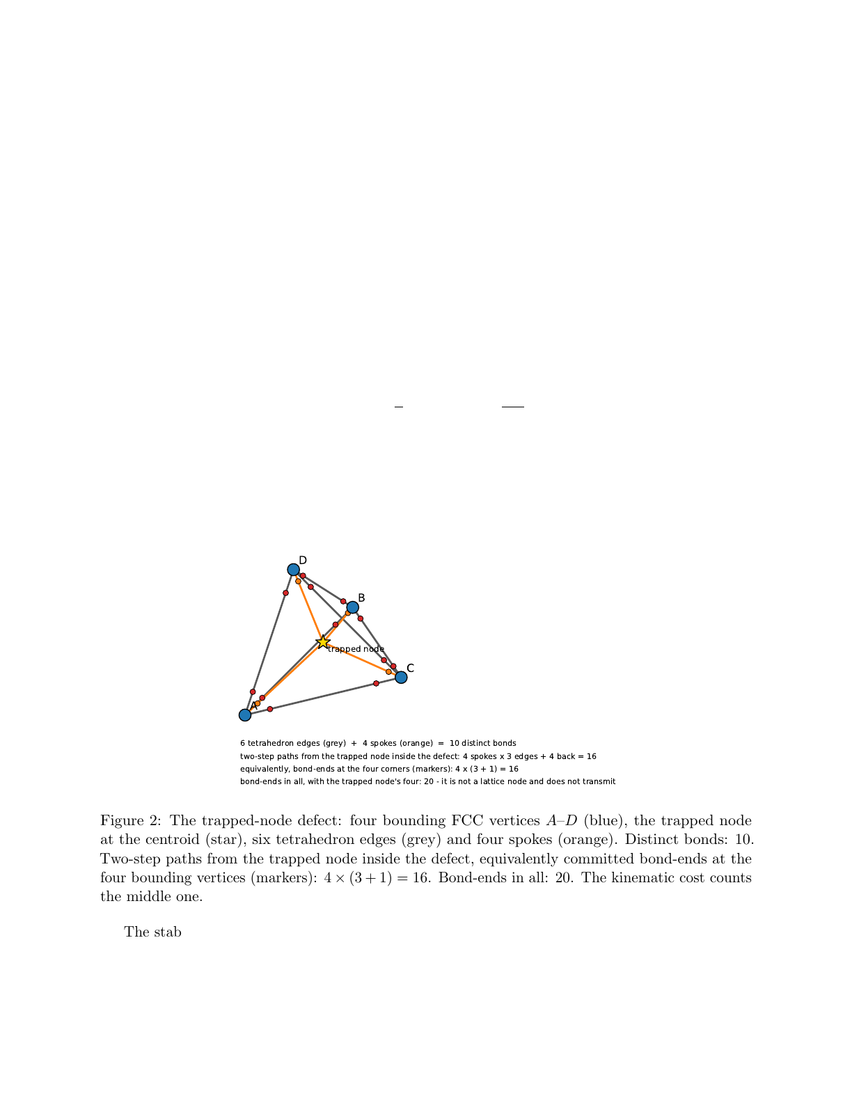
coordination shell, which has six members, but the number of two-step paths from a node, twelve
neighbors times twelve onward steps.
Its information cost is the number of such paths from its thirteen structural nodes into the bulk,
less the 36 that never leave the defect (Appendix E), (
K+
1)
K
2
− c
skew
K
= 13
×
144
−
36 = 1836,
one bit each by (P3): that is the mass count of Refs. [2, 3], m
p
c
2
= 1836 ϵ
b
.
Its kinematic cost is the number of two-step paths from the trapped node inside the defect.
Figure 2 shows the structure: a complete graph
K
4
on the four bounding vertices with four spokes to
the trapped node, six tetrahedron edges and four spokes, ten distinct bonds. From the trapped node
there are four spokes, each continuing along the three
K
4
edges at its corner, and four out-and-back
paths,
4 × 3 + 4 = 16, (19)
which is also the number of committed bond-ends at the four bounding vertices, four each, and
numerically (
K/d
)
2
. These paths are internal reconfigurations the code resolves within an update,
so (P4) prices them by (P2), one quantum per node per tick:
m
p
c
2
= 16
ℏ
τ
= 16 E
bond
=
4ℏc
L
c
. (20)
The convention is that of Ref. [
3
] itself: its “13 structural nodes” are the twelve corner ends of the
six edges plus the center. For the photon sector the priced object was a bond’s phase, one term per
bond; here it is a two-step path, priced as standing outside the defect and as transient inside it.
Which side of the defect boundary a path falls on is geometry; that the two sides are priced by (P3)
and (P2) respectively is (P4).
A
B
C
D
trapped node
6 tetrahedron edges (grey) + 4 spokes (orange) = 10 distinct bonds
two-step paths from the trapped node inside the defect: 4 spokes x 3 edges + 4 back = 16
equivalently, bond-ends at the four corners (markers): 4 x (3 + 1) = 16
bond-ends in all, with the trapped node's four: 20 - it is not a lattice node and does not transmit
Figure 2: The trapped-node defect: four bounding FCC vertices
A
–
D
(blue), the trapped node
at the centroid (star), six tetrahedron edges (grey) and four spokes (orange). Distinct bonds: 10.
Two-step paths from the trapped node inside the defect, equivalently committed bond-ends at the
four bounding vertices (markers): 4
×
(3 + 1) = 16. Bond-ends in all: 20. The kinematic cost counts
the middle one.
The stability window is the statement that the two costs coincide where the code is stable: 1836
external two-step paths at one bit each equal 16 internal ones at one quantum each. With both in
hand it is an equation, 1836
ϵ
b
= 16
E
bond
, one kinematic quantum at a defect end balancing 114
.
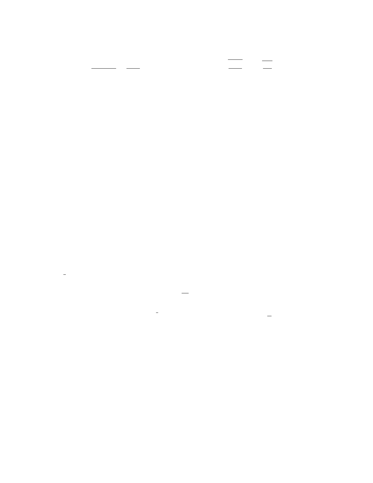
75
17
bits of disruption, and it fixes the confinement length with no length input:
L
c
=
16
¯
λ
e
4 × 1836
=
4
¯
λ
e
1836
= 0.8413 fm, α
−1
= 4π
r
1836
16
= π
r
m
p
m
e
= 134.6. (21)
The coupling is then a pure number from the code’s count and the FCC coordination, with
K/d
entering twice, once in E
bond
and once in the bond-end count, and L
c
has dropped out.
Now the comparison. The measured proton charge radius is 0
.
8409(4) fm, 0
.
05% from Eq.
(21)
;
the running coupling at 0
.
235 GeV is 135
.
5
±
0
.
3, 0
.
7% from it. Read the other way, as a check on
the count: writing the kinematic cost as
N E
bond
for general
N
gives
L
c
=
N
¯
λ
e
/
(4
×
1836), and
L
c
=
r
p
requires
N
= 15
.
99. The other natural integers of the geometry, 4 (the spokes), 10 (the
distinct bonds), 12 (
K
), 13 (
K+
1), 20 (all bond-ends), 24 (cuboctahedron edges), 36 (the verification
footprint of Ref. [
2
], a different object), give
L
c
= 0
.
21
,
0
.
53
,
0
.
63
,
0
.
68
,
1
.
05
,
1
.
26
,
1
.
89 fm; none
is within 18%. Equation
(21)
is Trinhammer and Bohr’s
r
p
= 4
ℏ/m
p
c
(Section 9) read inside the
model.
The construction rests on one counting object, ordered two-step paths from the defect’s nodes,
cut by the defect boundary and priced by (P4) with the two energies of (P2) and (P3). No measured
coupling enters it; the comparison above is with
r
p
, which the construction does not use. What it
does assume is that the trapped node itself does not transmit, being a defect rather than a lattice
node: counting its four ends as well would give
N
= 20 and
L
c
= 1
.
05 fm, as the list above shows.
The reading is therefore falsifiable by the model’s own bookkeeping, and it is the one the series
already uses.
8.12 The rotor’s monopoles
Compact
U
(1) has magnetic monopoles, and at
β ≃
11 they are ordinary objects of the Coulomb
phase. On the confinement code they are a consistency test. A unit monopole is a site of the
dual lattice with
div B
= 2
π
. At weak coupling its energy is the lattice Coulomb self-energy,
E
m
=
1
2
(2π)
2
v(0) J with v(0) =
R
d
3
k/(2π)
3
[
P
i
4 sin
2
(k
i
/2)]
−1
= 0.2527, so
E
m
= 4.98 J = 1.24
ℏc
L
c
= 292 MeV = 571 ϵ
b
(22)
on the confinement code (script alpha monopole.py). Three remarks.
The mass is hadronic, not exotic. It lies between
m
π
= 140 MeV and
√
σ
= 440 MeV, at the
scale of Λ
QCD
. Had it come out at a few GeV or below
m
π
, the model would owe an explanation of
why colliders and cosmic-ray searches have not seen it. It did not, and under (A2) the rotor is not
the propagating field, so its monopoles do not propagate in the fine code’s spacetime either.
What a monopole is in the code. A plaquette is one bond whose two paths disagree; a Dirac
string is a chain of such bonds; a monopole is where the chain ends. That is a defect of the kind the
sieve of Ref. [
2
] classifies. The pion of that paper is a two-sheet defect closed by a one-bond string,
at 273
ϵ
b
; the monopole’s 571
ϵ
b
is not a count in Table 2 of Ref. [
2
]. Whether the monopole is a
string-breaking state, a bound pair, or an object the sieve rejects, is open.
What it does not do. The number is a weak-coupling estimate and does not include the
monopole’s interaction with the Gauss-law charges or with the color code on the same lattice. It is
a check that the construction has no light exotic, not a prediction of a state.
18
9 Relation to earlier work
Six lines of work sit near this result. The paper should be read against them; the first three are
close enough in outcome that the differences in method are what matter.
Multiple Point Principle. Bennett and Nielsen take the fine-structure constants to be lattice-
scale quantities, compared with experiment through running, sitting at a multi-critical point of
lattice gauge theory; that gave
α
−1
= 137
±
9 [
20
]. Nielsen’s recent work takes the lattice as
ontological and places nine energy scales on a line against the power of the link length; the hadron
string scale, 0
.
42 GeV, is one of the points [
21
]. He calls that placement physically absurd, since a
cutoff should not know the hadron scale, and offers no mechanism. The present paper shares the
ontological lattice and the running comparison. It differs in mechanism: the coupling is a stiffness
ratio, not a critical value, and the lattice has two definite realizations rather than a fluctuating
spacing. Section 3.3 gives Nielsen’s observation a structural reading: the confinement scale is a
lattice scale because the vacuum crystallizes there.
Proton radius. Trinhammer and Bohr obtain
r
p
= 4
ℏ/
(
m
p
c
) = 0
.
841235641 fm from an intrinsic
toroidal configuration space [
22
]; it matches the muonic-hydrogen radius to 5
×
10
−4
. Equation
(9)
with L
c
= r
p
reads r
p
= 4π
2
α
2
¯
λ
e
. The two together give
m
p
m
e
=
1
π
2
α
2
, (23)
which holds to 1
.
3% with
α
at 0
.
235 GeV and to 3
.
6% with the Thomson value. The two relations
are compatible only with the running coupling. That is a cross-check of Section 5, not a competitor.
Section 8.11 then reads their identity inside the model:
m
p
c
2
= 4
ℏc/L
c
is the kinematic cost of the
sixteen internal two-step paths of the trapped-node defect at one quantum each, and the stability
window turns it into
L
c
= 4
¯
λ
e
/
1836. The model gives the identity an origin: the sixteen is a path
count on the defect graph and the pricing is (P2) and (P4), so
r
p
= 4
ℏ/m
p
c
is here a consequence
rather than a starting point.
The combination
π
p
m
p
/m
e
. Shchegolev [
26
] obtained
α
2
= (
m
e
/π
2
m
p
) (
E
R
/E
main
) from a
model of the proton as a freely precessing gyroscope, with
E
R
/E
main
= 1
/
1
.
036 a ratio of two
energies of his model. Without that factor the expression is
α
−1
=
π
p
m
p
/m
e
= 134
.
6, Eq.
(21)
; the
factor is what makes it 137
.
04. Two-thirds of it is vacuum polarization: (137
.
04
/
135
.
5)
2
= 1
.
023 is
the Standard Model running between zero momentum and the confinement scale, and the remaining
1
.
3% is the residual of Table 1. The combination therefore predates this paper; what is new is its
scale, its derivation from (P1)–(P5) rather than from a fitted energy ratio, and the identification of
most of the correction with the Standard Model running.
Emergent photons. That the coupling of an emergent
U
(1) is a computable function of a
microscopic stiffness ratio is the result of Hermele, Fisher and Balents [
23
] and Pace et al. [
10
]. This
paper applies that machinery to a vacuum lattice; the machinery is theirs, and Proposition 3 is the
cubic-lattice statement of their finding that low-level link variables give α ∼ 0.1.
Quantum link models and fracton phases. Gauge theories with finite-dimensional link Hilbert
spaces are the quantum link models of Horn, Orland and Rohrlich, and Chandrasekharan and
Wiese [
24
]; the spin-1 model of Proposition 3 is one. Gauge theories with subsystem conservation
19
laws and restricted mobility are the fracton phases of Vijay, Haah and Fu and the higher-rank
theories of Pretko [
25
]; the code’s own
U
(1) lift (Appendix E) belongs to that family, and the
cube-edge form of the code invites a comparison with cube-stabilizer codes that we have not pursued.
Numerology. Eddington, Wyler and their successors target 137
.
036 at zero momentum with no
mechanism. Section 5 shows that is the wrong target on either code. The present relation is stated
at a scale, carries a running, follows from stated axioms, and reads in both directions against a
second measured quantity.
10 The ledger
Table 2 collects the status of every claim, in the convention of Ref. [
5
] with one label added: identified,
a model quantity assigned to a role in a standard framework, stated rather than derived. No row
above rests on a measured coupling; the measured values appear as the calibrated and testable rows.
Table 2: Status of every claim in the paper.
status claim where
derived Maxwell structure of the ⟨100⟩ sector; exact incidence counts Sec. 4
derived
Counts are identical on both realizations (combinatorial–metric
principle)
Sec. 3.2
derived
A coupling that is a property of each realization is not a count;
the relation obtained contains L
c
and is not a count in any case
Prop. 1, Sec. 8.4
derived
The code’s checks are the parity of a
U
(1) cube-edge constraint;
that constraint is not the photon’s Gauss law (its lift is anisotropic,
non-Maxwell); the photon’s dual Gauss law is the tetrahedral-void
divergence (Maxwell to five figures)
Prop. 2
derived
Two- and three-level link variables give
α
−1
≈
7 and 14–30
(
L
= 6
,
8 and extrapolation), by projector Monte Carlo and exact
diagonalization; substantially more than three levels are needed
(fluctuation bound: at least seven), so the photon’s link variable
is rotor-like with small explicit U/J
Prop. 3
derived Edge-length field excluded by representation (spin-2) Sec. 6
derived
Ring-exchange flip amplitude 2
t
2
/V
in the auxiliary boson model
(J
KS
= 4t
2
/V )
App. B
derived 4 = K/d, given c = v
ph
of Ref. [6] Sec. 8.1
derived Scales U ∝ ϵ
b
, J ∝ E
bond
, from (P4) Sec. 8.8
derived u
= 1: the minimal charged excitation is one bond of flux (a
half-link’s flux is a charge–anticharge pair), and
ϵ
b
is the electron’s
cost with
C
e
= 1; the half-link reading would make the electron
half a bond
Sec. 8.8
derived ȷ
= 1: the flux current of the phase term is
I
=
−
(
J/ℏ
)
sin B
,
exact since [
H
J
, B
] = 0, so the maximum transfer per tick is
Jτ /ℏ
;
(P2) sets it to one quantum. The span and single-channel readings
give
1
2
and 2 quanta per tick
Sec. 8.8
derived Z
= (
ℏ/e
2
)
p
U/J
,
v
=
a
√
UJ/ℏ
, with no lattice-volume factor in
Z
App. D
derived
Rotor monopole mass
E
m
= 4
.
98
J
= 292 MeV at weak coupling;
hadronic, not exotic
Sec. 8.12
20

derived
The Hamiltonian in the model’s variables, Eq.
(10)
, structure
fixed by geometry; (P2) gives
J
=
ℏ/τ
on the per-bond term
with no bridge (the auxiliary form, Eq.
(24)
, is in Appendix B’s
normalization); no significant dressing of U/J by the tick within
the tested truncations (10
−4
single bond, 0
.
2–1% quartet, 1
.
7%
residual off the two-operator subspace)
Sec. 8.7
calibrated L
f
= 1.843 ℓ
P
to G
N
and the area law Ref. [5]
calibrated
Fine-code stiffnesses
U
f
= 0
.
68
E
bond,f
,
J
f
= 47
E
bond,f
, from the
impedance ratio and the condition
c
lat
=
c
; both are Planckian
and kinematic, as the fine code carrying no standing information
requires
Sec. 8.3
calibrated α
−1
(ℏc/L
f
) = 104.9 ± 0.3; α
−1
(ℏc/L
c
) = 135.5 ± 0.3 Sec. 5
calibrated
Kogut–Susskind relation checked by projector Monte Carlo at
L
= 4:
α
−1
= 132–136 for
U/J
= (4
πα
)
2
against 135
.
5 at tree
level
Sec. 8.6
derived N
= 16: one counting object, ordered two-step paths from the
defect’s nodes (
K
2
= 144 per node), priced as standing outside
(1836 = 13
×
144
−
36, one bit each, the
−
36 being the paths that
never leave the defect; enumerated in App. E) and transient inside
(16, one quantum each; Fig. 2); with the count 1836
ϵ
b
and the
stability equality this gives
L
c
= 0
.
8413 fm and
α
−1
=
π
p
m
p
/m
e
;
the alternatives (10, 20, 36) are excluded
Sec. 8.11
identified
(I1)
U
=
ϵ
b
and (I2)
J
=
E
bond
as the roles the two energies play
in Eq.
(4)
; their scales and coefficients are then derived (rows
above)
Sec. 8.1
assumed
(A0) Standing-information postulate and its complement (tran-
sient costs E
bond
); ϵ
b
one constant on both codes
Sec. 3.3, Ref. [4]
assumed
(A1) Impedance
Z
2
=
U/J
set on the confinement code, where
the ϵ
b
-scale stiffness exists; fine-code value is running
Sec. 8.3
assumed
(A2) Speed
v
2
=
UJ
set on the fine code; bare impedance contin-
uous across codes, dressed by the running (one field, one bare
Z
);
rotor’s own speed 0.017 c
Sec. 7, 8.3
assumed
(A3) The code’s Bell-pair phases are the flat staggered restriction
of the rotor’s primal connection
Def. 1
assumed
Two-code reading itself (minimal reading of the four size con-
straints)
Sec. 3.3
testable
If
L
c
=
r
p
exactly,
α
−1
(0
.
235
GeV
) = 134
.
65
±
0
.
05 in the rotor’s
scheme
Sec. 8.5
testable
Relation compatible only with the small proton radius (0
.
877 fm
gives 131.9)
Sec. 8.5
testable ȷ/u
= 1
.
00
±
0
.
02 from the measured
α
and
r
p
, against the derived
1; the excluded readings would give 95 and 190
Sec. 8.9
not derived
The axioms themselves: (P1)–(P3) are the earlier papers’, (P4)
and (P5) this paper’s
Sec. 2.1
not derived The code identity of the monopole Sec. 8.12
not derived O
(
α
) lattice renormalization of the coupling beyond the ten-
percent check
Sec. 8.6
not derived
The matching map: a fine-code rotor Hamiltonian returning
U
f
= 0.68 E
bond,f
, J
f
= 47 E
bond,f
Sec. 8.3
No row rests on a measured coupling. What the paper does not derive is the axioms, the
21

rotor premise (A3) under which the photon sector is a
U
(1) rotor at all, and the two-code reading
(A1)–(A2); these are the framework’s, and a model in which the fine code’s rotors had their own code
stiffnesses would need a separate mechanism to suppress
U/J
there by eleven orders of magnitude.
The principal open problem is the matching map: a fine-code rotor Hamiltonian returning the
stiffnesses of Section 8.3. It is the “origin of the gauge variables” item of Ref. [
7
], now with a definite
operator to construct.
11 Conclusions
Figure 3 draws the chain of the paper from the axioms to the measured coupling, with the ledger’s
not-derived items beside it. The rest of this section states it in words.
22
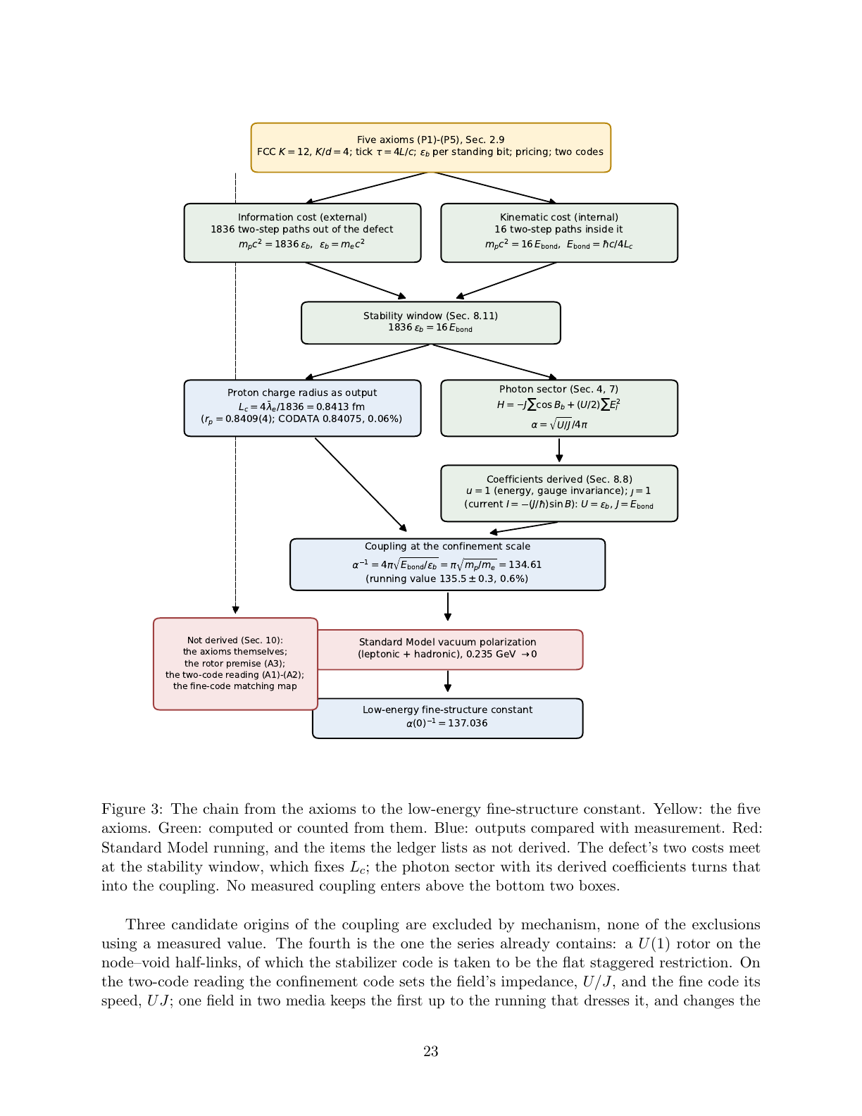
Five axioms (P1)-(P5), Sec. 2.9
FCC
K
= 12,
K
/
d
= 4; tick = 4
L
/
c
;
b
per standing bit; pricing; two codes
Information cost (external)
1836 two-step paths out of the defect
m
p
c
2
= 1836
b
,
b
=
m
e
c
2
Kinematic cost (internal)
16 two-step paths inside it
m
p
c
2
= 16
E
bond
,
E
bond
=
c
/4
L
c
Stability window (Sec. 8.11)
1836
b
= 16
E
bond
Proton charge radius as output
L
c
= 4
e
/1836 = 0.8413 fm
(
r
p
= 0.8409(4); CODATA 0.84075, 0.06%)
Photon sector (Sec. 4, 7)
H
=
J
cos
B
b
+ (
U
/2)
E
2
l
=
U
/
J
/4
Coefficients derived (Sec. 8.8)
u
= 1 (energy, gauge invariance); = 1
(current
I
= (
J
/ )sin
B
):
U
=
b
,
J
=
E
bond
Coupling at the confinement scale
1
= 4
E
bond
/
b
=
m
p
/
m
e
= 134.61
(running value 135.5 ± 0.3, 0.6%)
Standard Model vacuum polarization
(leptonic + hadronic), 0.235 GeV 0
Low-energy fine-structure constant
(0)
1
= 137.036
Not derived (Sec. 10):
the axioms themselves;
the rotor premise (A3);
the two-code reading (A1)-(A2);
the fine-code matching map
Figure 3: The chain from the axioms to the low-energy fine-structure constant. Yellow: the five
axioms. Green: computed or counted from them. Blue: outputs compared with measurement. Red:
Standard Model running, and the items the ledger lists as not derived. The defect’s two costs meet
at the stability window, which fixes
L
c
; the photon sector with its derived coefficients turns that
into the coupling. No measured coupling enters above the bottom two boxes.
Three candidate origins of the coupling are excluded by mechanism, none of the exclusions
using a measured value. The fourth is the one the series already contains: a
U
(1) rotor on the
node–void half-links, of which the stabilizer code is taken to be the flat staggered restriction. On
the two-code reading the confinement code sets the field’s impedance,
U/J
, and the fine code its
speed,
UJ
; one field in two media keeps the first up to the running that dresses it, and changes the
23
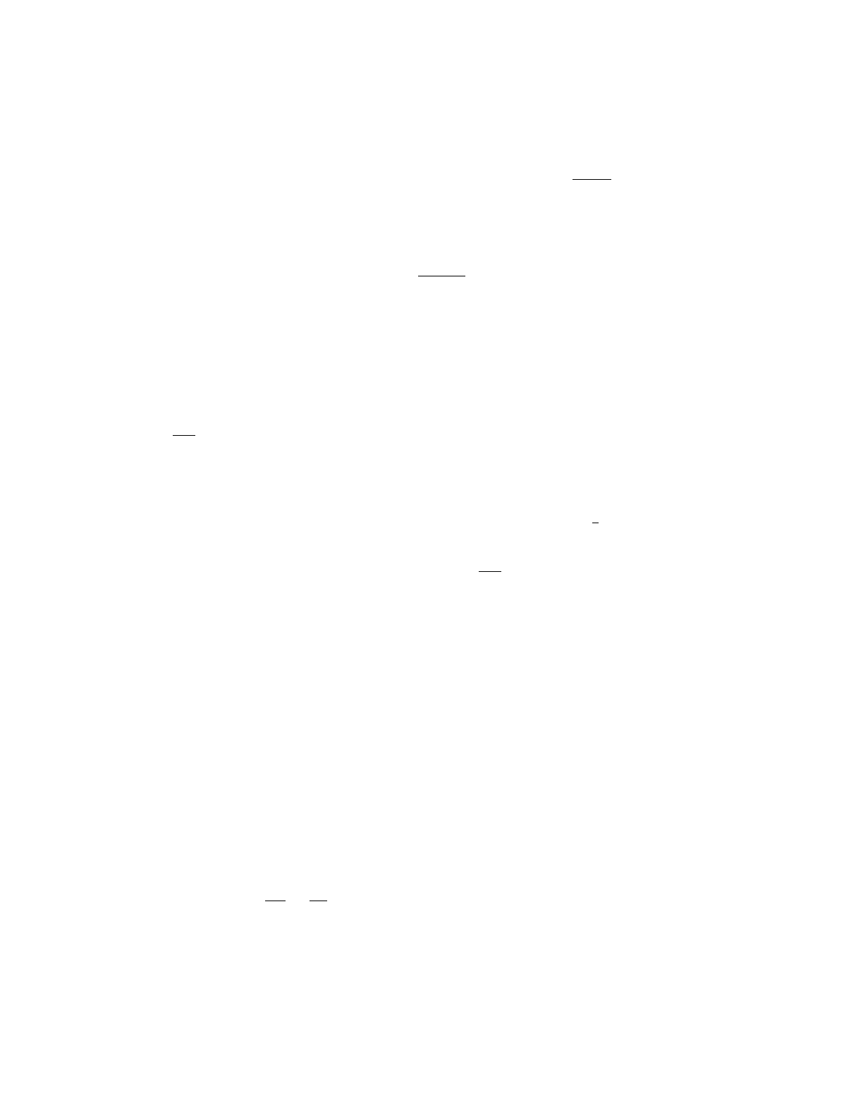
second. In the model’s own variables the Hamiltonian is a per-bond phase term and a four-bond
charging term. Its coefficients follow from (P2) and (P3) applied to the operators each postulate is
a statement about: the charging energy is one standing bit per bond of flux, the plaquette stiffness
one bond quantum, and the exact Floquet Hamiltonian of the tick shows no significant dressing of
their ratio. The coupling at the confinement scale is then
α
−1
= 2
π
p
¯
λ
e
/L
c
, a relation among the
fine-structure constant, the electron mass and the proton radius holding to 0
.
6% in
α
−1
with no
fitted parameter. The stability window, in kinematic form, removes
L
c
as well: one count applied
twice, two-step paths from the trapped-node defect, 1836 into the bulk at one bit each and 16 inside
it at one quantum each, equated where the code is stable. Within the SSM, then,
α
is not a free
parameter: from the axioms alone,
α
−1
=
π
p
m
p
/m
e
= 134
.
6, with the proton radius an output
(0
.
8413 against 0
.
8409 fm). The axioms themselves, the rotor premise and the two-code reading
remain the framework’s; the ledger of Section 10 lists them. The rotor’s monopoles come out at
292 MeV, hadronic rather than exotic, and the relation is compatible only with the small proton
radius.
A Running of the coupling
Two-loop
MS
running of
g
1
, g
2
, g
3
, y
t
from
µ
=
m
t
, with
g
1
in GUT normalization, one-loop
coefficients
b
= (41
/
10
, −
19
/
6
, −
7), two-loop gauge matrix
B
=
199/50 27/10 44/5
9/10 35/6 12
11/10 9/2 −26
, and Yukawa
coefficients (17
/
10
,
3
/
2
,
2):
dg
i
/d ln µ
=
g
3
i
(
b
i
+
P
j
B
ij
g
2
j
/
16
π
2
− C
i
y
2
t
/
16
π
2
)
/
16
π
2
. Inputs
g
1
=
0
.
4626
, g
2
= 0
.
6478
, g
3
= 1
.
1666
, y
t
= 0
.
9369 [
11
].
α
−1
em
= 4
π
(1
/g
2
2
+
5
3
/g
2
1
). Results at 6
.
62
×
10
18
GeV: 105
.
53 at one loop, 104
.
86 at two loops; 108
.
7 at 10
16
GeV. Two-loop sensitivities:
g
3
+1%,
+0
.
00;
g
1,2
+ 0
.
1%,
−
0
.
25;
y
t
+ 1%, +0
.
01. Below
m
t
, the value at
Q
= 0
.
235 GeV uses the exact
one-loop leptonic vacuum polarization (spacelike) or the
MS
logarithms, plus the hadronic estimate
quoted in the text; the two schemes bracket the quoted ±0.3.
B Ring exchange on the ⟨100⟩ lattice
This is the auxiliary primal boson realization referred to in Sections 7 and 8.8, in which the plaquette
term arises at second order; the model’s own variables, in which it is a per-bond term priced by
(P2), are treated in Sections 8.7 and 8.8. Hard-core bosons on the
⟨
100
⟩
links. Gauss law: three
of six links occupied at every site. Charge penalty
V
per unit
|div|
. Hopping
t
between links
sharing a site. Second-order degenerate perturbation theory on the twenty-link cluster of a plaquette
gives, for every flippable background, exactly four two-hop paths from a plaquette configuration
to its flip. Each passes through an intermediate carrying two unit charges, of cost 2
V
. Hence
J
= 4
× t
2
/
(2
V
) = 2
t
2
/V
for the amplitude of the flip operator
R
p
+
R
†
p
; since
R
p
+
R
†
p
= 2
cos B
p
in the rotor limit, the stiffness in the
cos B
normalization of Eq.
(4)
is
J
KS
= 2
J
= 4
t
2
/V
. The
Monte Carlo of Section 8.6 uses
J
KS
= 2
J
ring
. The normalization derived in Section 8.8 reads, in
this model,
4t
2
V
=
ℏc
4L
i.e. V = 4 E
bond
for t = E
bond
, (24)
a transient unit charge priced on the four
⟨
110
⟩
bonds the moved link serves, one quantum each.
The four is the served quartet of Section 4; pricing the charge per violated site instead (
V
= 2) or
per moved link (
V
= 1) would give
α
−1
= 190 and 269. This is the same statement as
ȷ
= 1, in this
realization’s language.
24
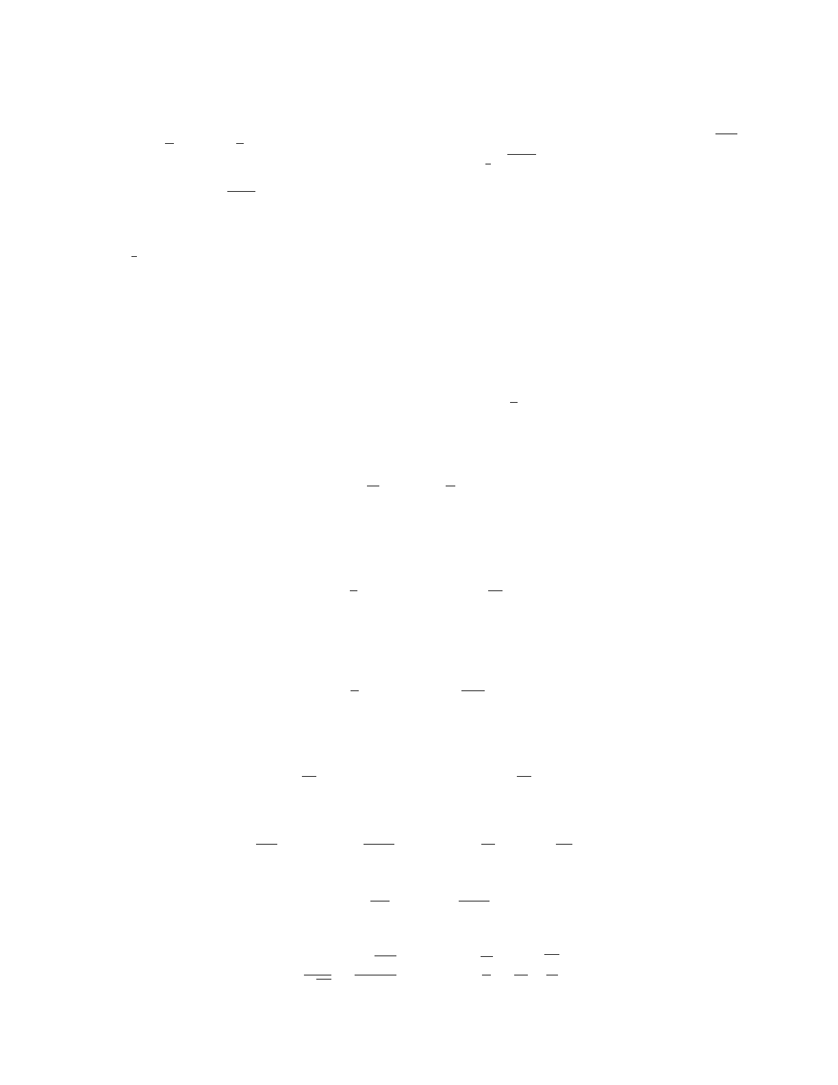
C The level bound and the Gaussian estimate
For
H
=
U
2
P
E
2
+
J
2
P
B
2
on the cubic link lattice, the transverse modes have
ω
k
=
λ
k
√
UJ
,
λ
2
k
=
P
i
4
sin
2
(
k
i
/
2), and ground-state fluctuation
⟨E
2
l
⟩
=
1
3
p
J/U ⟨λ⟩
BZ
with
⟨λ⟩
= 2
.
388. A link
with 2
S
+ 1 levels has
⟨E
2
⟩ ≤ S
2
, so for a given coupling this bounds the level count from below:
α
−1
= 135
.
5, i.e.
p
J/U
= 10
.
8, needs
⟨E
2
⟩ ≃
8
.
6 per link, hence
S ≥
2
.
9: at least seven levels of
the link variable, and more once the non-photon share of the fluctuation is included. Read the other
way, as an estimate of the coupling from a level count, the same relation is unreliable: applied to
spin-
1
2
quantum spin ice it gives
α
−1
= 3
.
7 against the literature
≃
10 [
10
], and applied to the spin-1
model of Section 6.2 it gives 54 against the Monte Carlo 14. The sum rule over
⟨E
2
⟩
is dominated
by short-wavelength, non-photon fluctuations whose share depends on the model. Only the bound
is used in the text; the couplings quoted for low-level variables are the direct Monte Carlo and
exact-diagonalization values of Proposition 3.
D Normalization of impedance and speed
Take the cubic link lattice of Section 4 with spacing
a
=
L/
√
2
, three links and three plaquettes
per site. The rotor variables are the link angle
θ
l
and its conjugate integer flux
E
l
, with
B
p
the
circulation of θ around a plaquette. In the harmonic regime, β ≫ 1, the Hamiltonian is
H =
U
2
X
l
E
2
l
+
J
2
X
p
B
2
p
. (25)
The dictionary to continuum fields fixes what
E
l
and
B
p
are.
E
l
is the electric flux through the
link’s dual plaquette in units of the charge quantum e, so with D the electric displacement,
E
l
=
1
e
Z
dual plaq
D · dA =
a
2
e
D
l
. (26)
θ
l
is the holonomy of the vector potential along the link,
θ
l
= (
e/ℏ
)
a A
l
, so
B
p
is the magnetic flux
through the plaquette in units of the flux quantum,
B
p
=
e
ℏ
Z
plaq
B · dA =
e a
2
ℏ
B
phys
p
. (27)
Sums over links and plaquettes become integrals with one factor of 1
/a
3
and one direction per link
or plaquette,
X
l
D
2
l
=
1
a
3
Z
d
3
x D
2
,
X
p
(B
phys
p
)
2
=
1
a
3
Z
d
3
x B
2
. (28)
Substituting,
H =
Ua
2e
2
Z
d
3
x D
2
+
Je
2
a
2ℏ
2
Z
d
3
x B
2
=
1
2ϵ
Z
D
2
+
1
2µ
Z
B
2
, (29)
which identifies
ϵ =
e
2
Ua
, µ =
ℏ
2
Je
2
a
. (30)
So U plays 1/ϵ in the D formulation, J plays 1/µ, and the two constants of the medium are
v =
1
√
ϵµ
=
a
√
UJ
ℏ
, Z =
r
µ
ϵ
=
ℏ
e
2
r
U
J
. (31)
25
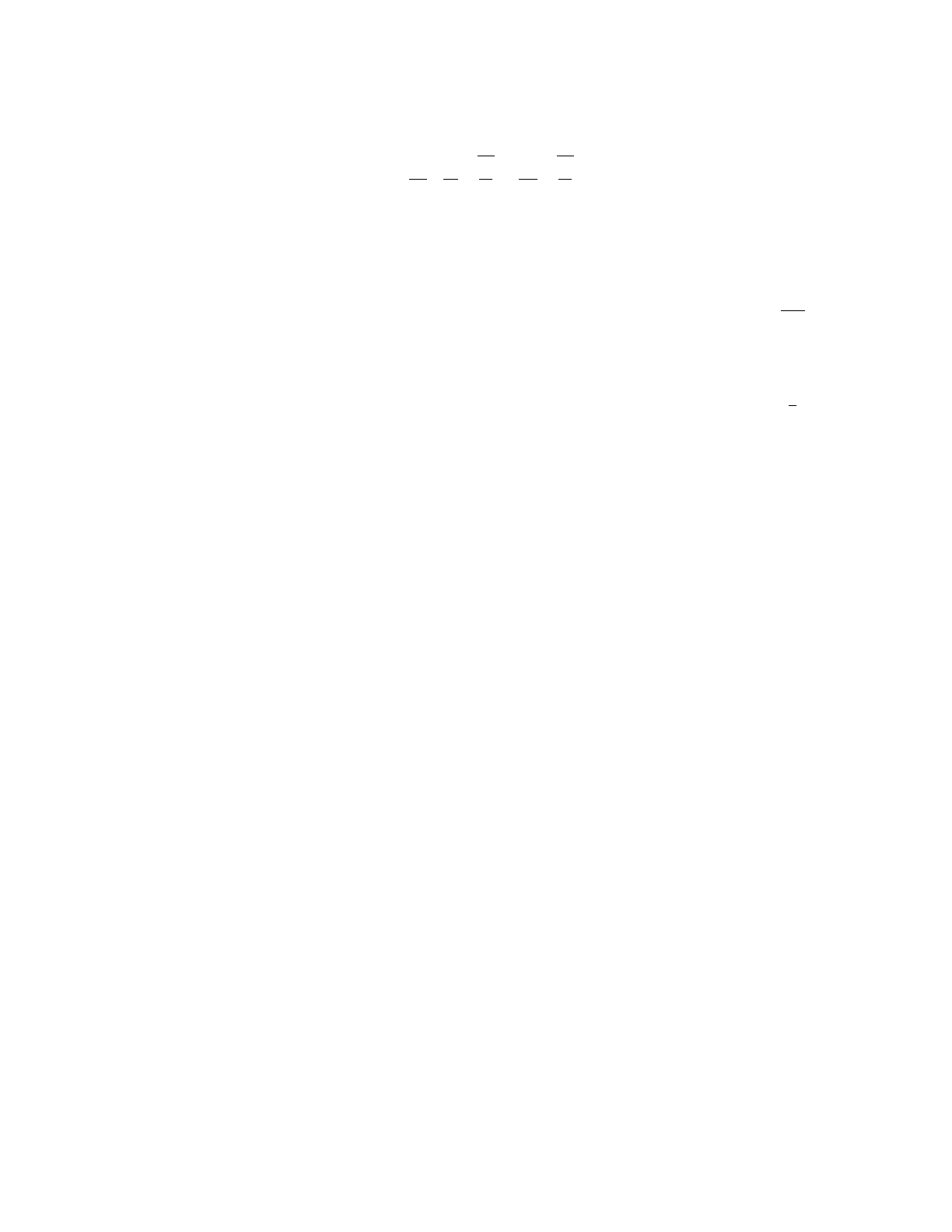
The spacing
a
enters the speed and cancels in the impedance. With
α
=
Ze
2
/
2
h
, the second of
these gives
α =
e
2
2h
·
ℏ
e
2
r
U
J
=
1
4π
r
U
J
, (32)
the Kogut–Susskind relation of Eq.
(4)
, now with its normalization explicit: unit
E
is one charge
quantum of flux, unit B is one flux quantum, and no lattice-volume factor survives.
For the cross-code matching of Section 8.3 this is what matters. The two codes have the same
combinatorics, so the per-site counts (three links, three plaquettes) and the dictionary above are
identical on both; only
a
differs. Equation
(31)
then says that the bare
Z
is the same on both
codes if and only if
U/J
is, with no geometric factor to track, while
v
carries
a
and
√
UJ
and
differs; the dressing of Eq.
(7)
multiplies
U/J
by (
α
f
/α
c
)
2
and is the only other factor. Had the
two lattices differed in coordination or cell shape, the identifications of
ϵ
and
µ
would each carry
a lattice-dependent constant and the matching condition would read (
U/J
)
f
=
γ
(
U/J
)
c
with
γ
computable from the two geometries; here γ = 1. The compact term −J cos B
p
reduces to
J
2
B
2
p
at
β ≃ 11 up to the renormalization checked at the ten-percent level in Section 8.6.
E The dual lattice and the two U(1) lifts: details
This appendix gives the structural results behind Section 4 and Propositions 2–3, the numerical
methods behind Sections 6.2, 8.6 and 8.7, and the two-step-path counts used in Section 8.11. Every
statement was verified by enumeration at N = 4 and N = 6 with the scripts of Appendix F.
The code as a cube-edge code. Each FCC bond is an edge of exactly two regular tetrahedra
whose centers differ by a unit
⟨
100
⟩
step, so the tetrahedral voids form a simple cubic lattice
D
with the bonds as its links. The eight tetrahedra around a node have exactly twelve unit-step edges
among them, the twelve bonds at that node; the eight around an octahedral void have as their twelve
edges the twelve bonds of the octahedron. Hence the
Z
-checks are the edges of the node-centerd
cubes of
D
and the
X
-checks the edges of the void-centerd cubes: the [[3
N
3
,
2
N
3
+ 2
,
3]] code is
a twelve-body cube-edge code on a simple cubic lattice.
D
is the Poincar´e dual of the node–void
lattice
P
: its links pierce the plaquettes of
P
, one per bond; its plaquettes are pierced by the links
of
P
and consist of the served quartets; its cubes are centerd on the sites of
P
, and its own sites are
the tetrahedral voids at which Ref. [3] places the trapped node of Section 8.11.
Counting. Over
F
2
the divergence-free link fields on
P
have dimension 2
N
3
+ 1; the code’s logical
dimension is 2
N
3
+ 2; the served-quartet map from bond fields to link fields is the transpose of
the curl of
P
, of rank 2
N
3
−
2 (the coexact dimension), never producing a harmonic mode, and
not descending to the logical quotient (an
X
-check maps to a weight-24 link field with nonzero
curl). The logical space is the space of bond fields obeying the mod-2 Gauss law at every node and
every void; it and the photon’s divergence-free space are different objects of dimensions 2
N
3
+ 2
and 2N
3
+ 1 (130 and 129 at N = 4; 434 and 433 at N = 6).
Lift A: the code’s checks as a
U
(1) Gauss law. Impose zero sum of integer bond variables
over the twelve edges of every cube of
D
. Over
R
the
N
3
cube sums have 3
N −
2 dependencies:
in each lattice plane the node-cube sums minus the void-cube sums vanish identically, since an
in-plane bond has all four of its cubes in the plane and a crossing bond one node and one void.
The constrained space has dimension 2
N
3
+ 3
N −
2. The elementary local move preserving every
cube sum is an alternating flip on a tetrahedral four-cycle, four of the six edges of one tetrahedral
26
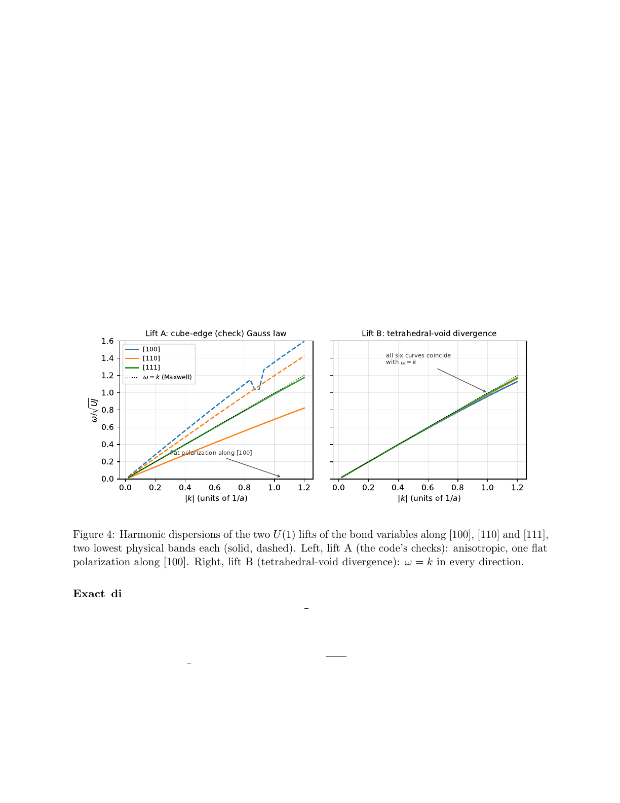
void omitting one skew pair, three per tetrahedron labeled by the omitted pair (the three colors of
Ref. [
3
]); the moves span 2
N
3
−
3
N
+ 1 dimensions, leaving 6
N −
3 planar subsystem invariants. A
four-cycle flip needs four single-bond moves through intermediates carrying four unit charges (eight
in one ordering of three), so ring exchange is fourth order, with flip amplitude (5
/
16)
t
4
/V
3
. The
harmonic Bloch spectrum (phases on bonds gauge-shifted by the cube constraints, four-cycle term
expanded) has
ω
2
/k
2
= 2 and 0 along [100], 0
.
5 and 1
.
5 along [110], 1 and 1 along [111], 0
.
28 and
1
.
72 along [210] (Fig. 4, left). Lift A is a subsystem-symmetric gauge theory with a flat polarization
along the axes, in the family of Refs. [25]; it is not Maxwell.
Lift B: the tetrahedral-void divergence. Orient each bond from one of its tetrahedra to the
other and impose zero signed divergence at every tetrahedral void. The primal electric field on a
link is the oriented circulation of the bond field around the dual plaquette the link pierces, and is
divergence-free identically; this is the Villain dual of Maxwell on
P
. The elementary move is an
alternating flip on a served quartet, moving one unit of primal flux across a site; ring exchange is
second order, with flip amplitude 2
t
2
/V
, i.e.
J
KS
= 4
t
2
/V
(Appendix B). The harmonic dispersion
is
ω
2
/k
2
= 0
.
99997, 0
.
99998, 0
.
99999, 0
.
99998, 0
.
99998 for both polarizations along [100], [110],
[111], [210], [321] at |k| = 0.02 (Fig. 4, right).
0.0 0.2 0.4 0.6 0.8 1.0 1.2
|
k
| (units of 1/
a
)
0.0
0.2
0.4
0.6
0.8
1.0
1.2
1.4
1.6
/
UJ
flat polarization along [100]
Lift A: cube-edge (check) Gauss law
[100]
[110]
[111]
=
k
(Maxwell)
0.0 0.2 0.4 0.6 0.8 1.0 1.2
|
k
| (units of 1/
a
)
all six curves coincide
with =
k
Lift B: tetrahedral-void divergence
Figure 4: Harmonic dispersions of the two
U
(1) lifts of the bond variables along [100], [110] and [111],
two lowest physical bands each (solid, dashed). Left, lift A (the code’s checks): anisotropic, one flat
polarization along [100]. Right, lift B (tetrahedral-void divergence): ω = k in every direction.
Exact diagonalization. Lift B on a 2
×
2
×
2 periodic cubic lattice (24 links). Gauss-law
sectors enumerated by meet-in-the-middle: spin-
1
2
, 4248 states at winding zero and 2352 at winding
one; spin-1, 1 676 839 and 1 289 360. Electric stiffness from
E
0
(
W =
1)
− E
0
(0) =
U/
2
L
; magnetic
stiffness from the curvature of
E
0
(
θ
) under a phase twist on the plaquettes crossing a boundary,
by second-order perturbation theory (validated against finite differences to four digits). Ground
energies −9.0267 (spin-
1
2
) and −20.1476 (spin-1);
p
J/U = 0.405 and 0.992.
Projector Monte Carlo. Since all off-diagonal elements of
−H
are +
J
, the ground state is
positive in the flux basis. Power-method projector
G
= 1
−
∆
τ
(
H − E
T
) with ∆
τ
= 0
.
3
/N
plaq
,
adaptive
E
T
, stochastic reconfiguration every ten steps, ancestry tracked for forward walking. The
27
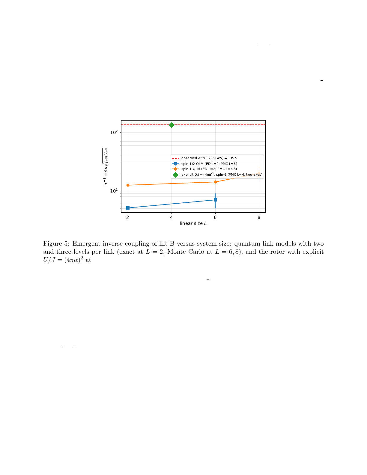
transverse structure factor
S
T
(k) =
⟨|E
T
(k)
|
2
⟩
at the smallest k gives
p
J/U
=
S
T
/λ
k
directly.
Ground energies at
L
= 2:
−
9
.
012(26) and
−
20
.
123(39) against the exact values. Spin-1: at
L
= 6
the three axes give
S
T
/λ
= 1
.
12
,
1
.
06
,
1
.
20 (
α
−1
= 13–15); at
L
= 8, 1
.
44
,
2
.
25
,
1
.
19 (15–28), a
spread that reflects forward-walking lineage collapse, quoted as 20
±
6; the drift from
L
= 6 to 8
is a finite-
k
correction, and extrapolation in
k
2
puts the infinite-volume value near 25–30. Spin-
1
2
at
L
= 6: 7. Explicit charging energy: Section 8.6 (Fig. 5). At
L
= 6 with an explicit charging
energy the forward-walking lineages collapse over the required projection time and the estimator
degenerates to the mixed one; a worldline method with pure estimators is needed there.
2 4 6 8
linear size
L
10
1
10
2
1
= 4
J
eff
/
U
eff
observed
1
(0.235 GeV) = 135.5
spin-1/2 QLM (ED L=2; PMC L=6)
spin-1 QLM (ED L=2; PMC L=6,8)
explicit
U
/
J
= (4 )
2
, spin-6 (PMC L=4, two axes)
Figure 5: Emergent inverse coupling of lift B versus system size: quantum link models with two
and three levels per link (exact at
L
= 2, Monte Carlo at
L
= 6
,
8), and the rotor with explicit
U/J
= (4
πα
)
2
at
L
= 4 (two lattice axes). Dashed: the observed coupling at the confinement scale.
The tick unitary. With
U
τ
=
exp
(
ig
P
b
cos B
b
)
exp
(
−
i
2
ϵ
P
l
(
curl m
)
2
l
) in the flux basis (
|m| ≤
8
for a single bond,
|m| ≤
3 per bond for a served quartet),
H
F
=
i log U
τ
is projected onto the two
operators of Eq.
(10)
in the Hilbert–Schmidt sense. Single bond,
g
= 1,
ϵ
= 0
.
0087:
U
eff
/J
eff
equals
ϵ/g
to 10
−4
, and the induced two-step hopping is 10
−4
. Served quartet at
g
= 0
.
3
,
0
.
5
,
0
.
7 (so that
4
g < π
and the logarithm is on its principal branch): ratios 0
.
998, 0
.
995, 0
.
990 of the input, residual
off the two-operator subspace 1.7%, truncation-limited.
Two-step paths. The counts of Section 8.11 are of ordered two-step paths on the bond graph, and
alpha two step.py
enumerates them. From an FCC node there are
K
2
= 144, twelve neighbors
times twelve onward steps; twelve return to the origin and the rest reach 54 distinct endpoints, so
K
2
is a path count and not a shell count (the second coordination shell has six members). The defect’s
four bounding vertices are four distinct lattice nodes, each an end of three of the tetrahedron’s six
edges, so the “13 structural nodes” of Ref. [
3
] are twelve corner ends plus the trapped center, and
the external leading term is 13
×
144 = 1872 ordered paths. Inside the defect, whose graph is
K
4
on
the four bounding vertices with four spokes to the center, the two-step paths from the trapped node
are four spokes times three
K
4
edges at the corner reached, plus four out-and-back, 4
×
3 + 4 = 16;
equivalently, four committed bond-ends at each of the four bounding vertices.
The correction is the same enumeration continued. Of the paths counted above, those that
never leave the defect are not external: from each bounding vertex there are three first steps along
28
tetrahedron edges and three second steps from wherever each lands, 4
×
3
×
3 = 36 ordered paths in
all, twelve of them returning to their starting corner. Removing them gives
13 × 144 − 36 = 1836, (33)
which is Ref. [
3
]’s (
K+
1)
K
2
− c
skew
K
with
c
skew
K
= 3
×
12 = 36 recovered as the internal-path
count. The external and internal counts of Section 8.11 are therefore one enumeration with one
cut, the defect boundary: 1836 paths that leave it, priced as standing, and 16 from the trapped
node that stay inside, priced as transient. The cut matters at the two-percent level and is what
makes the result sharp: 13
×
144 = 1872 without it would give
L
c
= 0
.
8251 fm, 1
.
9% below
r
p
, and
α
−1
= π
√
1872 = 135.9, against 0.8413 fm and 134.6 with it.
What the tick unitary would add. Section 8.8 fixes the two coefficients from what (P2) and
(P3) are statements about, applied to the two kinds of operator in Eq.
(10)
. It does not construct
the tick from the code’s own dynamics. That construction, a quantum cellular automaton on the
bonds with one step per
τ
, built from the operations the series names (the stitch and lift kinematics
of Ref. [
3
], syndrome extraction on every cube of
D
, the standing-bit cost of Ref. [
4
]), would settle
two things this paper assumes rather than derives: that the photon sector is a
U
(1) rotor at all (the
premise (A3) of Section 7), and the fine-code stiffnesses of Section 8.3, whose matching map is the
last not derived row of the ledger. It would also test the coefficients independently: an automaton
whose generator norms disagreed with
u
=
ȷ
= 1 would contradict Section 8.8 and, through Eq.
(18)
,
the measured coupling. It is not constructed here.
F Scripts
alpha run.py: two-loop running (Section 5, Appendix A).
alpha cost ratios.py: verification-cost ratios (Section 6).
alpha liftB gfmc.py
,
alpha liftB gfmc fast.py
: projector Monte Carlo for the photon
sector with finite-level link variables and, optionally, an explicit charging energy; forward-
walked transverse structure factor (Proposition 3, Section 8.6). The compiled version is
checkpointed.
alpha liftB ed.py
(with
alpha liftB ed common.py
): exact diagonalization
at L = 2 with electric and magnetic twists.
alpha liftB ice.py
: the photon’s charge-free ensemble with
Z
M
bond fluxes (classical
sampling, for the level bound).
alpha liftA liftB.py
: Bloch dispersion of the two
U
(1) lifts on the bonds (Proposition 2, Ap-
pendix E);
alpha dual moves.py
,
alpha dual spectrum.py
,
alpha logical vs photon.py
:
lift A’s moves, invariants and spectrum, and the counting identities.
alpha ice quartet.py: the cube-edge-constrained ensemble, for comparison.
alpha elastic projection.py: phonon projection (Section 6).
alpha ring exchange.py: ring exchange (Appendix B).
alpha gaussian levels.py
,
alpha calibrate diamond.py
: Gaussian estimate and its diamond-
lattice calibration (Appendix C).
alpha tick floquet.py
: exact Floquet Hamiltonian of the tick unitary;
U
eff
/J
eff
versus input
(Section 8.7).
29
alpha current operator.py
: the flux current of the phase term and the transfer per tick
(Section 8.8).
alpha two step.py: the two-step path counts of Section 8.11 (Appendix E).
alpha monopole.py: lattice monopole self-energy (Section 8.12).
alpha figures.py: Figs. 1–3.
The structural, running, Gaussian and Floquet scripts run with
numpy
/
scipy
in seconds to a
minute; the exact diagonalization takes minutes; the projector Monte Carlo takes minutes at
L
= 4 and hours per seed at
L ≥
6, and its compiled version needs
numba
. Archived at
https:
//github.com/raghu91302/ssmtheory/blob/main/alpha_scripts_v2.zip.
Data availability
The scripts reproducing every computation in this paper are archived at
https://github.com/
raghu91302/ssmtheory/blob/main/alpha_scripts_v2.zip (Appendix F).
Declaration of competing interest
The author declares no conflict of interest.
References
[1]
R. Kulkarni, A 67%-rate CSS code on the FCC lattice: [[192
,
130
,
3]] from weight-12 stabilizers,
arXiv:2603.20294 (2026).
[2]
R. Kulkarni, The mass–energy–information equivalence: a bottom-up identification of
the particle spectrum via FCC lattice error correction, Phys. Open 27 (2026) 100414.
doi:10.1016/j.physo.2026.100414
[3]
R. Kulkarni, Matter as incomplete crystallization: quark charges, color confinement, and the
proton mass from a single extra node in the vacuum lattice, Phys. Open 27 (2026) 100423.
doi:10.1016/j.physo.2026.100423
[4]
R. Kulkarni, Dark matter as incomplete crystallization: a geometric construction on the octahe-
dral void of the FCC vacuum lattice, Quantum Rep. 8 (2026) 89. doi:10.3390/quantum8030089
[5]
R. Kulkarni, Black holes in the FCC selection–stitch model: Bekenstein–Hawking entropy,
geometric evaporation, and primordial-black-hole signatures, Eur. Phys. J. Plus 141 (2026) 916.
doi:10.1140/epjp/s13360-026-08148-9
[6]
R. Kulkarni, A two-step quantum–classical threshold at 13.1–22.6
µ
g with exact ratio
√
3
from
a close-packed vacuum lattice, Quantum Rep. 8 (2026) 78. doi:10.3390/quantum8030078
[7]
R. Kulkarni, Centrosymmetry, bipartiteness, and the photon polarization count on close-packed
lattices, submitted to Symmetry (2026), manuscript symmetry-4576823.
[8]
J. Kogut, L. Susskind, Hamiltonian formulation of Wilson’s lattice gauge theories, Phys. Rev.
D 11 (1975) 395. doi:10.1103/PhysRevD.11.395
30

[9]
A. H. Guth, Existence proof of a nonconfining phase in four-dimensional U(1) lattice gauge the-
ory, Phys. Rev. D 21 (1980) 2291, doi:10.1103/PhysRevD.21.2291; T. A. DeGrand, D. Toussaint,
Phys. Rev. D 22 (1980) 2478, doi:10.1103/PhysRevD.22.2478.
[10]
S. D. Pace, S. C. Morampudi, R. Moessner, C. R. Laumann, Emergent fine struc-
ture constant of quantum spin ice is large, Phys. Rev. Lett. 127 (2021) 117205.
doi:10.1103/PhysRevLett.127.117205
[11]
D. Buttazzo, G. Degrassi, P. P. Giardino, G. F. Giudice, F. Sala, A. Salvio, A. Stru-
mia, Investigating the near-criticality of the Higgs boson, JHEP 12 (2013) 089.
doi:10.1007/JHEP12(2013)089
[12]
OPAL Collaboration, G. Abbiendi et al., Measurement of the running of the QED coupling in
small-angle Bhabha scattering at LEP, Eur. Phys. J. C 45 (2006) 1. doi:10.1140/epjc/s2005-
02389-3
[13]
F. Jegerlehner, The Anomalous Magnetic Moment of the Muon, 2nd ed., Springer (2017).
doi:10.1007/978-3-319-63577-4
[14]
A. Antognini et al., Proton structure from the measurement of 2S–2P transition frequencies of
muonic hydrogen, Science 339 (2013) 417. doi:10.1126/science.1230016
[15]
P. J. Mohr, D. B. Newell, B. N. Taylor, E. Tiesinga, CODATA recommended val-
ues of the fundamental physical constants: 2022, Rev. Mod. Phys. 97 (2025) 025002.
doi:10.1103/RevModPhys.97.025002
[16]
LHAASO Collaboration, Z. Cao et al., Ultrahigh-energy photons up to 1.4 petaelectronvolts
from 12 γ-ray Galactic sources, Nature 594 (2021) 33. doi:10.1038/s41586-021-03498-z
[17]
V. Vasileiou et al., Constraints on Lorentz invariance violation from Fermi-Large
Area Telescope observations of gamma-ray bursts, Phys. Rev. D 87 (2013) 122001.
doi:10.1103/PhysRevD.87.122001
[18]
S. Navas et al. (Particle Data Group), Review of particle physics, Phys. Rev. D 110 (2024)
030001. doi:10.1103/PhysRevD.110.030001
[19]
G. S. Bali, QCD forces and heavy quark bound states, Phys. Rep. 343 (2001) 1.
doi:10.1016/S0370-1573(00)00079-X
[20]
D. L. Bennett, H. B. Nielsen, Gauge couplings calculated from multiple point criticality
yield
α
−1
= 137
±
9: at last, the elusive case of U(1), Int. J. Mod. Phys. A 14 (1999) 3313.
doi:10.1142/S0217751X99001524
[21]
H. B. Nielsen, Remarkable scale relation, approximate SU(5), fluctuating lattice, Uni-
verse 11 (2025) 211, doi:10.3390/universe11070211; Ontological fluctuating lattice cut off,
arXiv:2510.18517 (2025).
[22]
O. L. Trinhammer, H. G. Bohr, On proton charge radius definition, EPL 128 (2019) 21001.
doi:10.1209/0295-5075/128/21001
[23]
M. Hermele, M. P. A. Fisher, L. Balents, Pyrochlore photons: the U(1) spin liquid
in a
S
= 1
/
2 three-dimensional frustrated magnet, Phys. Rev. B 69 (2004) 064404.
doi:10.1103/PhysRevB.69.064404
31

[24]
D. Horn, Finite matrix models with continuous local gauge invariance, Phys. Lett. B 100
(1981) 149, doi:10.1016/0370-2693(81)90763-2; P. Orland, D. Rohrlich, Lattice gauge magnets:
local isospin from spin, Nucl. Phys. B 338 (1990) 647, doi:10.1016/0550-3213(90)90646-U;
S. Chandrasekharan, U.-J. Wiese, Quantum link models: a discrete approach to gauge theories,
Nucl. Phys. B 492 (1997) 455, doi:10.1016/S0550-3213(97)80041-7.
[25]
S. Vijay, J. Haah, L. Fu, Fracton topological order, generalized lattice gauge theory, and
duality, Phys. Rev. B 94 (2016) 235157, doi:10.1103/PhysRevB.94.235157; M. Pretko, Subdi-
mensional particle structure of higher rank U(1) spin liquids, Phys. Rev. B 95 (2017) 115139,
doi:10.1103/PhysRevB.95.115139.
[26] V. Shchegolev, A model of the proton, arXiv:physics/0506125 (2005).
32
